This function plots the aggregated residuals of k-fold cross-validated models against the outcome. This allows to evaluate how the model performs according over- or underestimation of the outcome.
Arguments
- data
A data frame, used to split the data into
ktraining-test-pairs.- formula
A model formula, used to fit linear models (
lm) over allktraining data sets. Usefitto specify a fitted model (also other models than linear models), which will be used to compute cross validation. Iffitis not missing,formulawill be ignored.- k
Number of folds.
- fit
Model object, which will be used to compute cross validation. If
fitis not missing,formulawill be ignored. Currently, only linear, poisson and negative binomial regression models are supported.
Details
This function, first, generates k cross-validated test-training
pairs and
fits the same model, specified in the formula- or fit-
argument, over all training data sets.
Then, the test data is used to predict the outcome from all
models that have been fit on the training data, and the residuals
from all test data is plotted against the observed values (outcome)
from the test data (note: for poisson or negative binomial models, the
deviance residuals are calculated). This plot can be used to validate the model
and see, whether it over- (residuals > 0) or underestimates
(residuals < 0) the model's outcome.
Examples
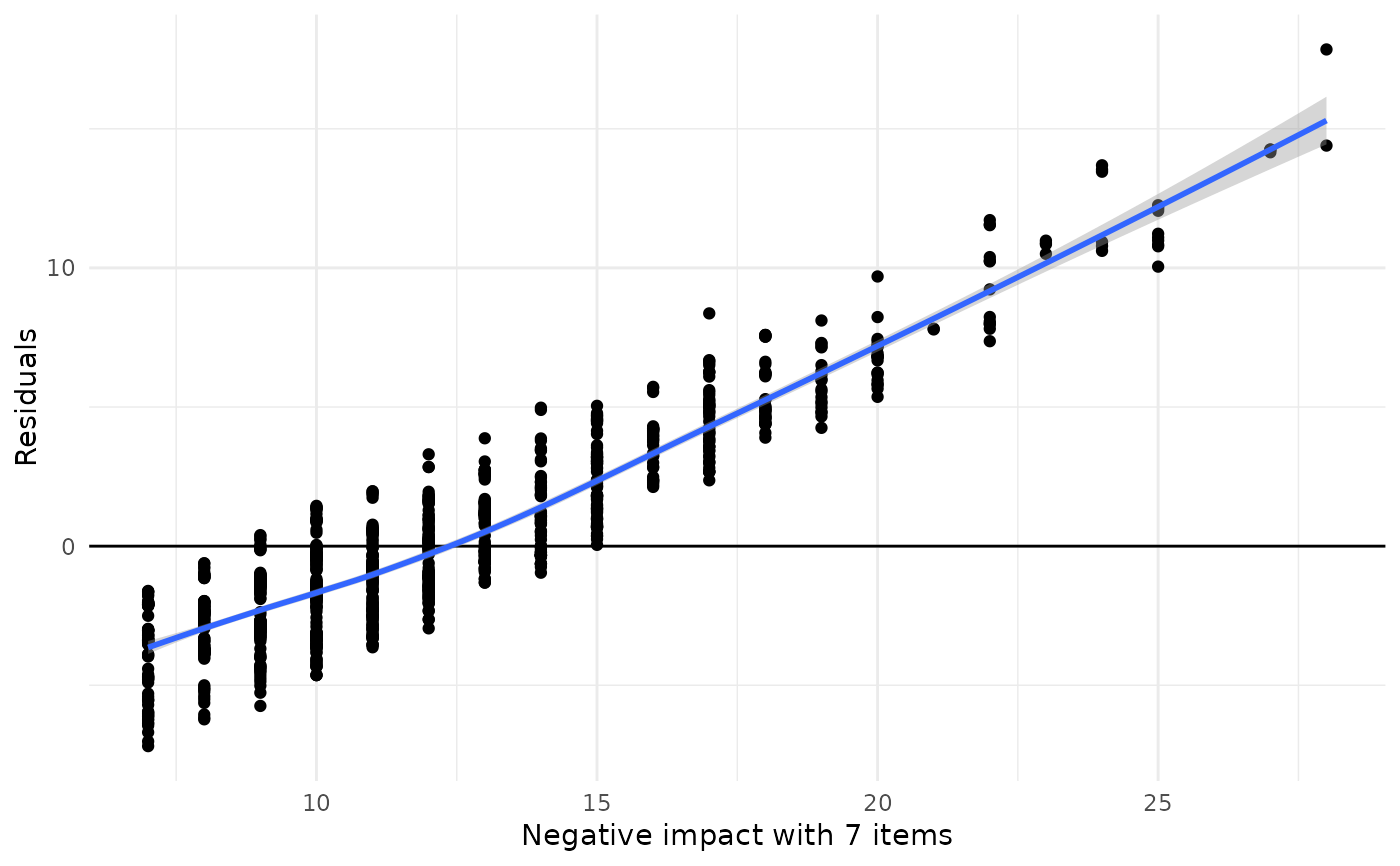
data(efc)
plot_kfold_cv(efc, neg_c_7 ~ e42dep + c172code + c12hour)
#> `geom_smooth()` using formula = 'y ~ x'
#> Warning: Removed 117 rows containing non-finite outside the scale range
#> (`stat_smooth()`).
#> Warning: Removed 117 rows containing missing values or values outside the scale range
#> (`geom_point()`).
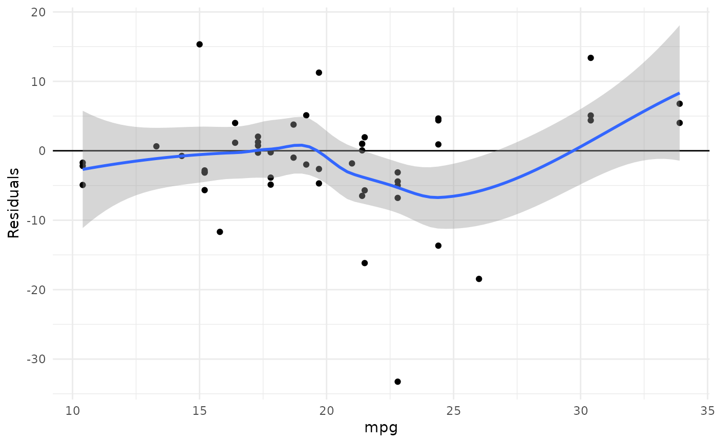
 plot_kfold_cv(mtcars, mpg ~.)
#> `geom_smooth()` using formula = 'y ~ x'
plot_kfold_cv(mtcars, mpg ~.)
#> `geom_smooth()` using formula = 'y ~ x'
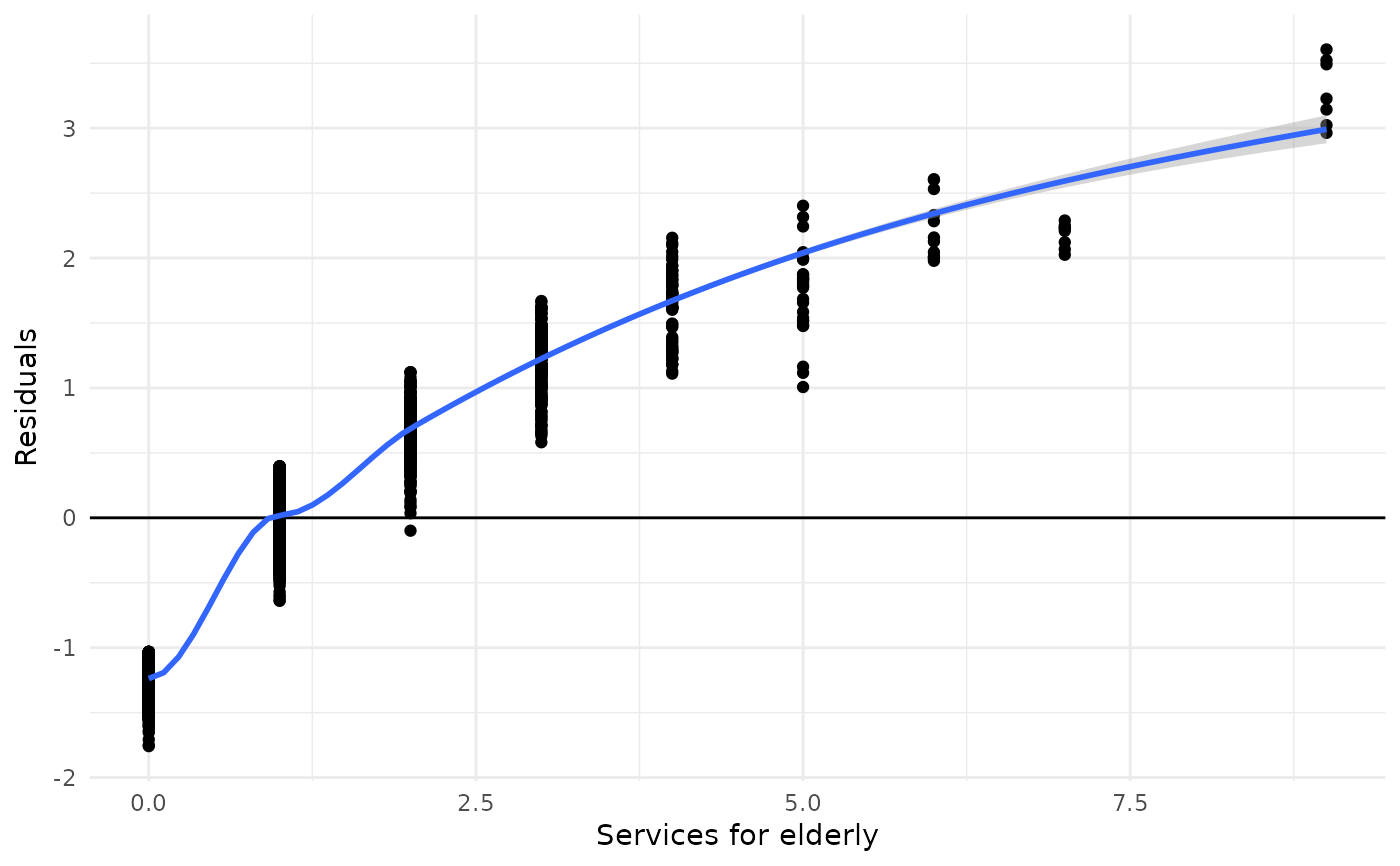
 # for poisson models. need to fit a model and use 'fit'-argument
fit <- glm(tot_sc_e ~ neg_c_7 + c172code, data = efc, family = poisson)
plot_kfold_cv(efc, fit = fit)
#> `geom_smooth()` using formula = 'y ~ x'
#> Warning: pseudoinverse used at -0.045
#> Warning: neighborhood radius 1.045
#> Warning: reciprocal condition number 0
#> Warning: There are other near singularities as well. 1
#> Warning: pseudoinverse used at -0.045
#> Warning: neighborhood radius 1.045
#> Warning: reciprocal condition number 0
#> Warning: There are other near singularities as well. 1
# for poisson models. need to fit a model and use 'fit'-argument
fit <- glm(tot_sc_e ~ neg_c_7 + c172code, data = efc, family = poisson)
plot_kfold_cv(efc, fit = fit)
#> `geom_smooth()` using formula = 'y ~ x'
#> Warning: pseudoinverse used at -0.045
#> Warning: neighborhood radius 1.045
#> Warning: reciprocal condition number 0
#> Warning: There are other near singularities as well. 1
#> Warning: pseudoinverse used at -0.045
#> Warning: neighborhood radius 1.045
#> Warning: reciprocal condition number 0
#> Warning: There are other near singularities as well. 1
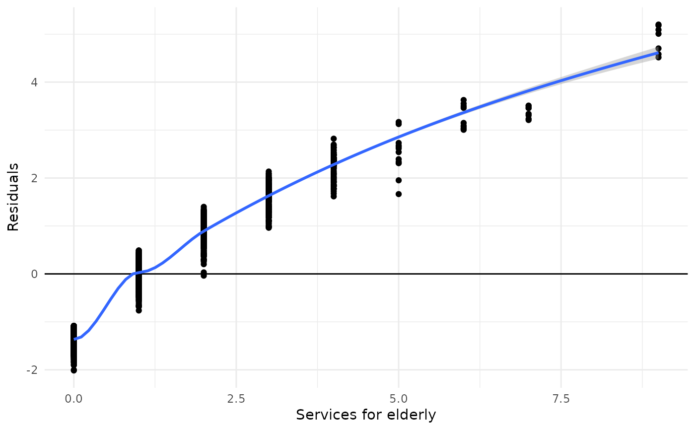 # and for negative binomial models
fit <- MASS::glm.nb(tot_sc_e ~ neg_c_7 + c172code, data = efc)
plot_kfold_cv(efc, fit = fit)
#> `geom_smooth()` using formula = 'y ~ x'
#> Warning: pseudoinverse used at -0.045
#> Warning: neighborhood radius 1.045
#> Warning: reciprocal condition number 1.0154e-30
#> Warning: There are other near singularities as well. 1
#> Warning: pseudoinverse used at -0.045
#> Warning: neighborhood radius 1.045
#> Warning: reciprocal condition number 1.0154e-30
#> Warning: There are other near singularities as well. 1
# and for negative binomial models
fit <- MASS::glm.nb(tot_sc_e ~ neg_c_7 + c172code, data = efc)
plot_kfold_cv(efc, fit = fit)
#> `geom_smooth()` using formula = 'y ~ x'
#> Warning: pseudoinverse used at -0.045
#> Warning: neighborhood radius 1.045
#> Warning: reciprocal condition number 1.0154e-30
#> Warning: There are other near singularities as well. 1
#> Warning: pseudoinverse used at -0.045
#> Warning: neighborhood radius 1.045
#> Warning: reciprocal condition number 1.0154e-30
#> Warning: There are other near singularities as well. 1