Introduction: Adjusted Predictions And Marginal Means At Specific Values • ggeffects

## Error in get(paste0(generic, ".", class), envir = get_method_env()) : 
##   object 'type_sum.accel' not found

Adjusted predictions and marginal means at specific values or levels

This vignettes shows how to calculate adjusted predictions at specific values or levels for the terms of interest. It is recommended to read the general introduction first, if you haven’t done this yet.

The terms-argument not only defines the model terms (i.e. focal variables) of interest, but each model term can be limited to certain “meaningful” (or “representative”) values. This allows to compute and plot adjusted predictions for (grouping) terms at specific values only, or to define values for the main effect of interest.

Summary of most important points:

The terms argument is not only used to define the focal terms, but also allows to specify meaningful values, at which predictions are calculated.
terms can be a character vector, a list, a formula, or a data frame. If a character vector, the values for the focal terms are placed in square brackets directly after the term name.
Although providing a list is probably the most R-native way to define the focal terms and meaningful values, providing a character vector additionally allows to use pre-defined "shortcuts". That's why this is the preferred way demonstrated throughout the package-documentation.
Non-focal terms can be fixed at specific values using the condition argument.

There are several options to define these meaningful values:

A character vector, specifying the names of the focal terms. This is the preferred and probably most flexible way to specify focal terms.
A list, where each element is a named vector, specifying the focal terms and their values. This is the “classical” R way to specify focal terms.
A formula, e.g. terms = ~ x + z, which is internally converted to a character vector. This is probably the least flexible way, as you cannot specify representative values for the focal terms.
A data frame representig a “data grid” or “reference grid”. Predictions are then made for all combinations of the variables in the data frame.

When terms is specified as character vector, values always should be placed in square brackets directly after the term name and can vary for each model term. The following examples show how to specify values for the terms-argument.

Concrete values are separated by a comma: terms = "c172code [1,3]". For factors, you could also use factor levels, e.g. terms = "Species [setosa,versicolor]". If terms is a named list, it would be specified like this: terms = list(c172code = c(1, 3)) or terms = list(c172code = c(1, 3), Species = c("setosa", "versicolor")). As a data frame, this would be:

terms <- data.frame(
  c172code = c(1, 3, 1, 3),
  Species = c("setosa", "setosa", "versicolor", "versicolor"),
  stringsAsFactors = FALSE
)
terms
#>   c172code    Species
#> 1        1     setosa
#> 2        3     setosa
#> 3        1 versicolor
#> 4        3 versicolor

Ranges are specified with a colon: terms = c("c12hour [30:80]", "c172code [1,3]"). This would plot all values from 30 to 80 for the variable c12hour. By default, the step size is 1, i.e. [1:4] would create the range 1, 2, 3, 4. You can choose different step sizes with by, e.g. [1:4 by=.5]. As named list, this would be terms = list(c12hour = 30:80) or terms = list(c12hour = seq(1, 4, 0.5)).
Convenient shortcuts to calculate common values like mean +/- 1 SD (terms = "c12hour [meansd]"), quartiles (terms = "c12hour [quartiles]") or minumum and maximum values (terms = "c12hour [minmax]"). See values_at() for the different options.
A function name. The function is then applied to all unique values of the indicated variable, e.g. terms = "hp [exp]". You can also define own functions, and pass the name of it to the terms-values, e.g. terms = "hp [own_function]".
A variable name. The values of the variable are then used to define the terms-values, e.g. first, a vector is defined: v = c(1000, 2000, 3000) and then, terms = "income [v]".
If the first variable specified in terms is a numeric vector, for which no specific values are given, a “pretty range” is calculated (see pretty_range()), to avoid memory allocation problems for vectors with many unique values. To select all values, use the [all]-tag, e.g. terms = "mpg [all]". If a numeric vector is specified as second or third variable in term (i.e. if this vector represents a grouping structure), representative values (see values_at()) are chosen, which is typically mean +/- SD.
To create a pretty range that should be smaller or larger than the default range (i.e. if no specific values would be given), use the n-tag, e.g. terms = "age [n=5]" or terms = "age [n = 12]". Larger values for n return a larger range of predicted values.
Especially useful for plotting group levels of random effects with many levels, is the sample-option, e.g. terms = "Subject [sample=9]", which will sample nine values from all possible values of the variable Subject.

Specific values and value range

library(ggeffects)
library(ggplot2)
data(efc, package = "ggeffects")
fit <- lm(barthtot ~ c12hour + neg_c_7 + c161sex + c172code, data = efc)

mydf <- predict_response(fit, terms = c("c12hour [30:80]", "c172code [1,3]"))
mydf
#> # Predicted values of Total score BARTHEL INDEX
#> 
#> c172code: low level of education
#> 
#> c12hour | Predicted |       95% CI
#> ----------------------------------
#>      30 |     67.15 | 64.03, 70.26
#>      38 |     65.12 | 62.05, 68.19
#>      47 |     62.84 | 59.80, 65.88
#>      55 |     60.81 | 57.77, 63.86
#>      63 |     58.79 | 55.72, 61.86
#>      80 |     54.48 | 51.28, 57.69
#> 
#> c172code: high level of education
#> 
#> c12hour | Predicted |       95% CI
#> ----------------------------------
#>      30 |     68.58 | 65.41, 71.76
#>      38 |     66.56 | 63.39, 69.73
#>      47 |     64.28 | 61.08, 67.48
#>      55 |     62.25 | 59.00, 65.50
#>      63 |     60.23 | 56.90, 63.55
#>      80 |     55.92 | 52.38, 59.46
#> 
#> Adjusted for:
#> * neg_c_7 = 11.84
#> * c161sex =  1.76
ggplot(mydf, aes(x, predicted, colour = group)) + geom_line()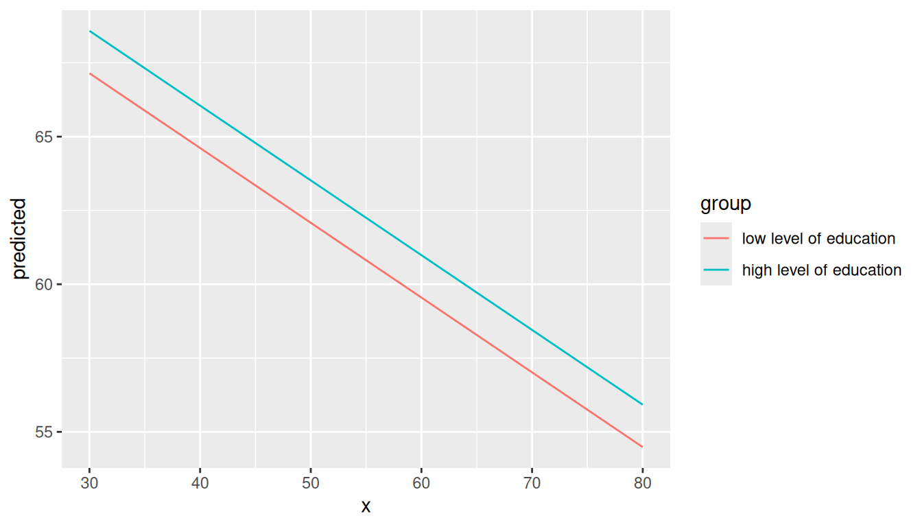

When variables are, for instance, log-transformed, ggeffects automatically back-transforms predictions to the original scale of the response and predictors, making the predictions directly interpretable. However, sometimes it might be useful to define own value ranges. In such situation, specify the range in the terms-argument.

data(mtcars)
mpg_model <- lm(mpg ~ log(hp), data = mtcars)

# x-values and predictions based on the full range of the original "hp"-values
predict_response(mpg_model, "hp")
#> # Predicted values of mpg
#> 
#>  hp | Predicted |       95% CI
#> ------------------------------
#>  50 |     30.53 | 27.84, 33.22
#>  85 |     24.82 | 23.21, 26.42
#> 120 |     21.11 | 19.91, 22.30
#> 155 |     18.35 | 17.11, 19.59
#> 195 |     15.88 | 14.36, 17.41
#> 230 |     14.10 | 12.29, 15.92
#> 265 |     12.58 | 10.48, 14.68
#> 335 |     10.06 |  7.45, 12.66

# x-values and predictions based on "hp"-values ranging from 50 to 150
predict_response(mpg_model, "hp [50:150]")
#> # Predicted values of mpg
#> 
#>  hp | Predicted |       95% CI
#> ------------------------------
#>  50 |     30.53 | 27.84, 33.22
#>  63 |     28.04 | 25.86, 30.23
#>  75 |     26.17 | 24.33, 28.00
#>  87 |     24.57 | 23.00, 26.13
#> 100 |     23.07 | 21.71, 24.43
#> 113 |     21.75 | 20.52, 22.99
#> 125 |     20.67 | 19.49, 21.84
#> 150 |     18.71 | 17.49, 19.92

By default, the step size for a range is 1, like 50, 51, 52, .... If you need a different step size, use by=<stepsize> inside the brackets, e.g. "hp [50:60 by=.5]". This would create a range from 50 to 60, with .5er steps.

# range for x-values with .5-steps
predict_response(mpg_model, "hp [50:60 by=.5]")
#> # Predicted values of mpg
#> 
#>    hp | Predicted |       95% CI
#> --------------------------------
#> 50.00 |     30.53 | 27.84, 33.22
#> 51.50 |     30.21 | 27.59, 32.84
#> 52.50 |     30.01 | 27.42, 32.59
#> 53.50 |     29.80 | 27.26, 32.34
#> 55.00 |     29.50 | 27.02, 31.98
#> 56.50 |     29.22 | 26.79, 31.64
#> 57.50 |     29.03 | 26.64, 31.41
#> 60.00 |     28.57 | 26.28, 30.86

Choosing representative values

Especially in situations where we have two continuous variables in interaction terms, or where the “grouping” variable is continuous, it is helpful to select representative values of the grouping variable - else, predictions would be made for too many groups, which is no longer helpful when interpreting adjusted predictions.

You can use

"minmax": minimum and maximum values (lower and upper bounds) of the variable are used.
"meansd": uses the mean value as well as one standard deviation below and above mean value.
"zeromax": is similar to the "minmax" option, however, 0 is always used as minimum value. This may be useful for predictors that don’t have an empirical zero-value.
"terciles" calculates and uses the terciles (lower, middle and upper), including minimum and maximum value.
"terciles2" calculates and uses the terciles (lower, middle and upper), excluding minimum and maximum value.
"threenum" calculates a three-number-summary (lower-hinge, median, and upper-hinge).
"fivenum" calculates Tukey’s five-number-summary (minimum, lower-hinge, median, upper-hinge, maximum).
"percentile" (including the percentile-value) calculates a range of values from the given percentile, e.g. "percentile80".
"all" takes all values of the vector.

data(efc, package = "ggeffects")
# short variable label, for plot
attr(efc$c12hour, "label") <- "hours of care"
fit <- lm(barthtot ~ c12hour * c161sex + neg_c_7, data = efc)

mydf <- predict_response(fit, terms = c("c161sex", "c12hour [meansd]"))
plot(mydf)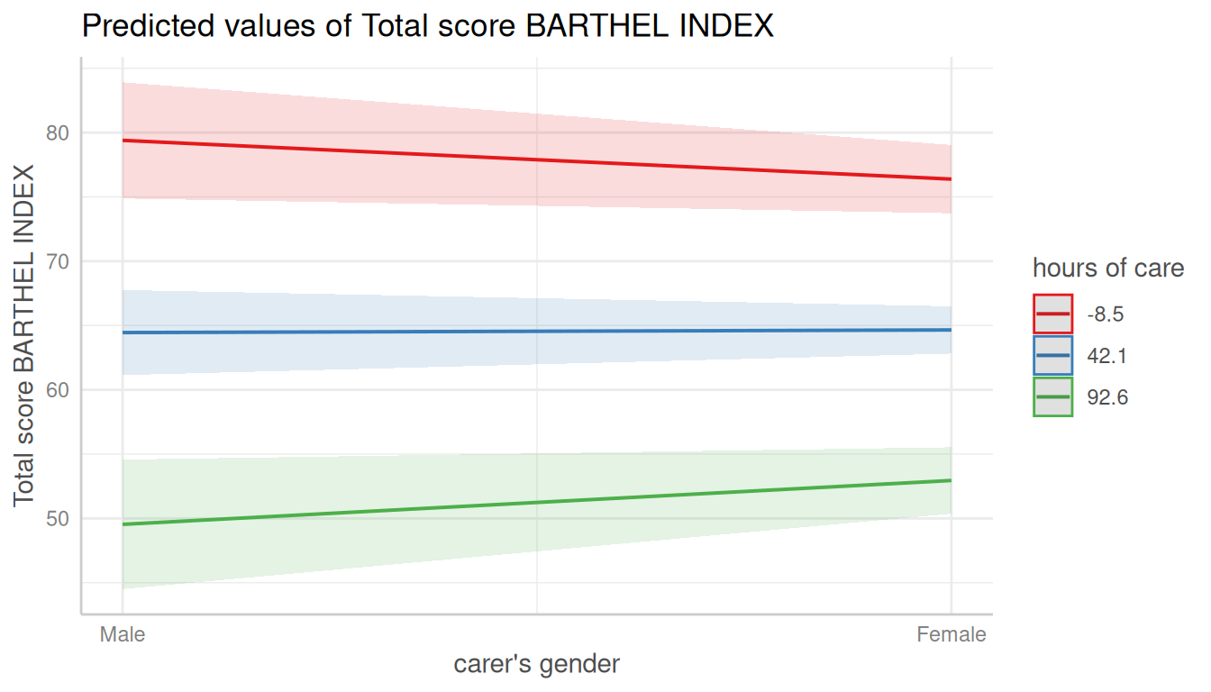


mydf <- predict_response(fit, terms = c("c161sex", "c12hour [quartiles]"))
plot(mydf)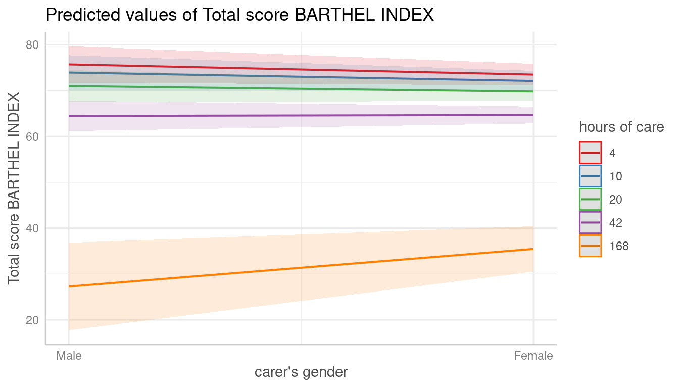

Transforming values with functions

The brackets in the terms-argument also accept the name of a valid function, to (back-)transform predicted values. In this example, we define a custom function to get the original values of the focal predictor, multiplied by 2.

# x-values and predictions based on "hp"-values, multiplied by 2
hp_double <- function(x) 2 * x
predict_response(mpg_model, "hp [hp_double]")
#> # Predicted values of mpg
#> 
#>     hp | Predicted |       95% CI
#> ---------------------------------
#> 104.00 |     22.65 | 21.34, 23.96
#> 132.00 |     20.08 | 18.91, 21.25
#> 186.00 |     16.39 | 14.94, 17.84
#> 210.00 |     15.08 | 13.43, 16.73
#> 226.00 |     14.29 | 12.51, 16.08
#> 300.00 |     11.24 |  8.88, 13.61
#> 410.00 |      7.88 |  4.81, 10.95
#> 670.00 |      2.59 | -1.63,  6.82

Using a list, the terms argument in the above example would look like this: terms = list(hp = hp_double(seq(100, 700, 7))).

Using values from a variable (vector)

val <- c(100, 200, 300)
predict_response(mpg_model, "hp [val]")
#> # Predicted values of mpg
#> 
#>  hp | Predicted |       95% CI
#> ------------------------------
#> 100 |     23.07 | 21.71, 24.43
#> 200 |     15.61 | 14.04, 17.17
#> 300 |     11.24 |  8.88, 13.61

Using a list, the terms argument in the above example would look like this: terms = list(hp = val).

Pretty value ranges

This section is intended to show some examples how the plotted output differs, depending on which value range is used. Some transformations, like polynomial or spline terms, but also quadratic or cubic terms, result in many predicted values. In such situation, predictions for some models lead to memory allocation problems. That is why predict_response() “prettifies” certain value ranges by default, at least for some model types (like mixed models).

To see the difference in the “curvilinear” trend, we use a quadratic term on a standardized variable.

library(datawizard)
library(lme4)
data(efc, package = "ggeffects")

efc$c12hour <- standardize(efc$c12hour)
efc$e15relat <- to_factor(efc$e15relat)

m <- lmer(
  barthtot ~ c12hour + I(c12hour^2) + neg_c_7 + c160age + c172code + (1 | e15relat),
  data = efc
)

me <- predict_response(m, terms = "c12hour")
plot(me)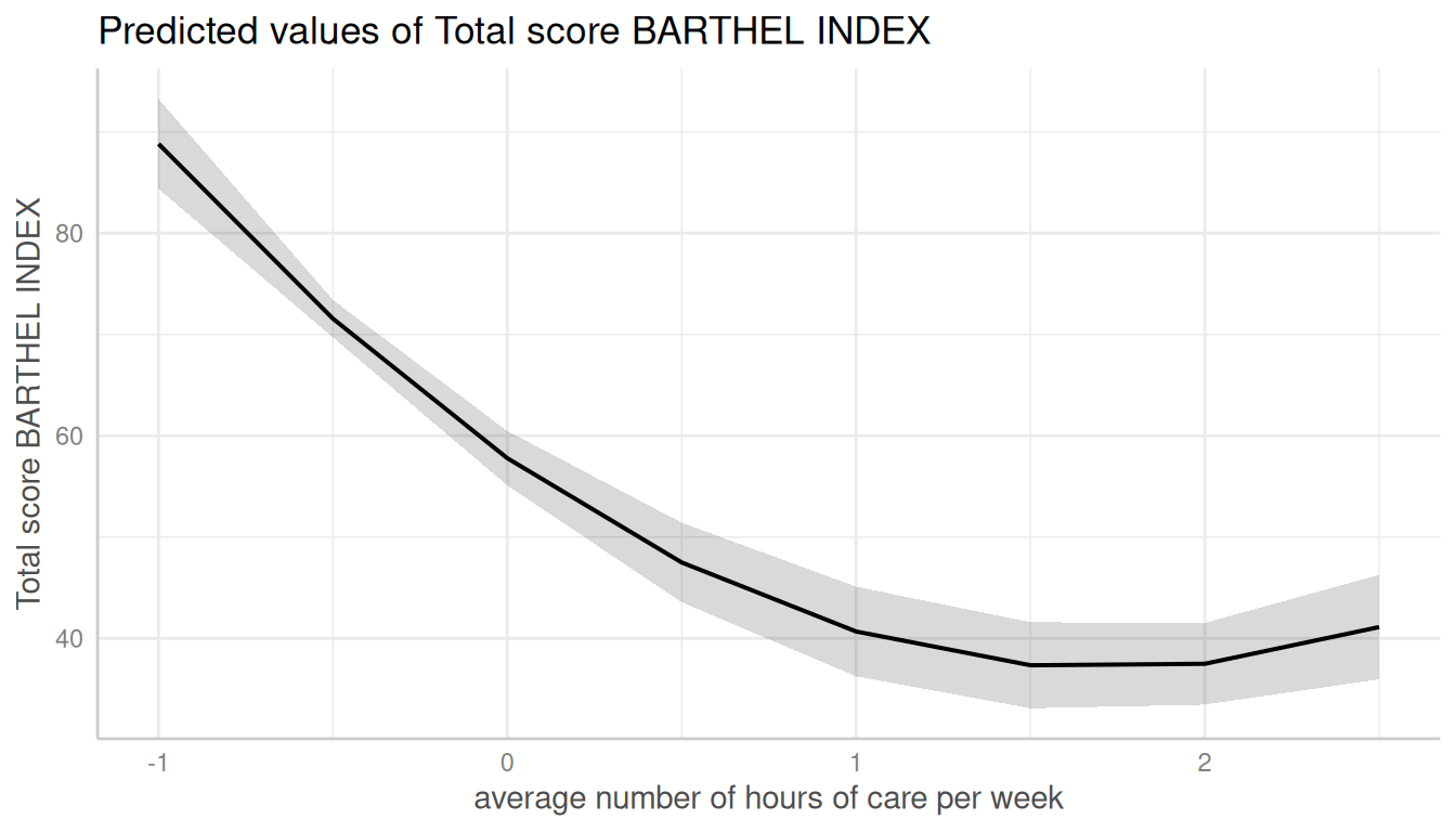

Turn off “prettifying”

As said above, predict_response() “prettifies” the vector, resulting in a smaller set of unique values. This is less memory consuming and may be needed especially for more complex models.

You can turn off automatic “prettifying” by adding the "all"-shortcut to the terms-argument.

me <- predict_response(m, terms = "c12hour [all]")
plot(me)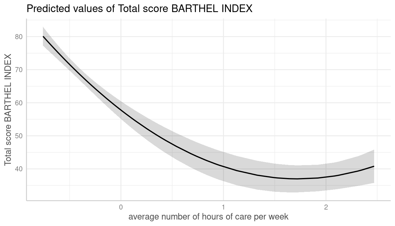

This results in a smooth plot, as all values from the term of interest are taken into account.

Using different ranges for prettifying

To modify the “prettifying”, add the "n"-shortcut to the terms-argument. This allows you to select a feasible range of values that is smaller (and hence less memory consuming) them "terms = ... [all]", but still produces smoother plots than the default prettyfing.

me <- predict_response(m, terms = "c12hour [n=2]")
plot(me)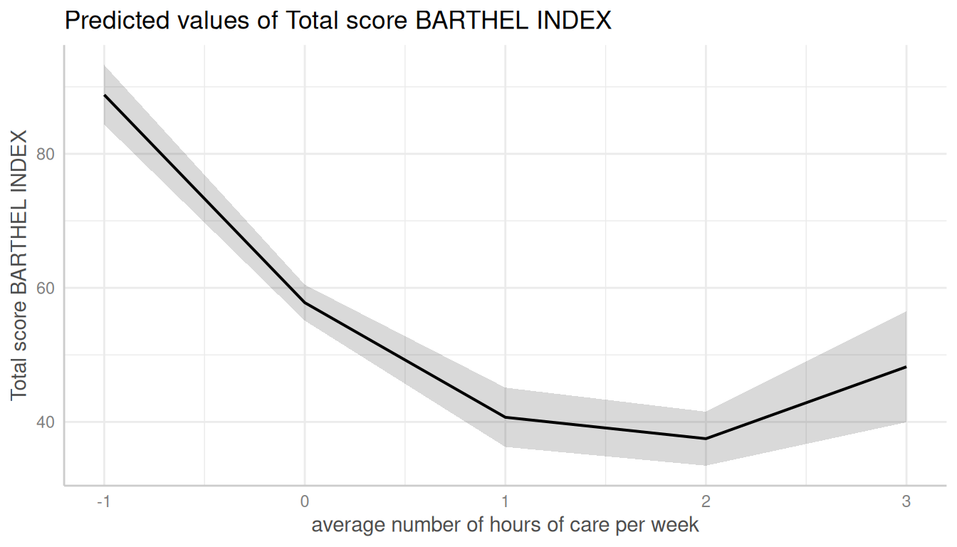

me <- predict_response(m, terms = "c12hour [n=10]")
plot(me)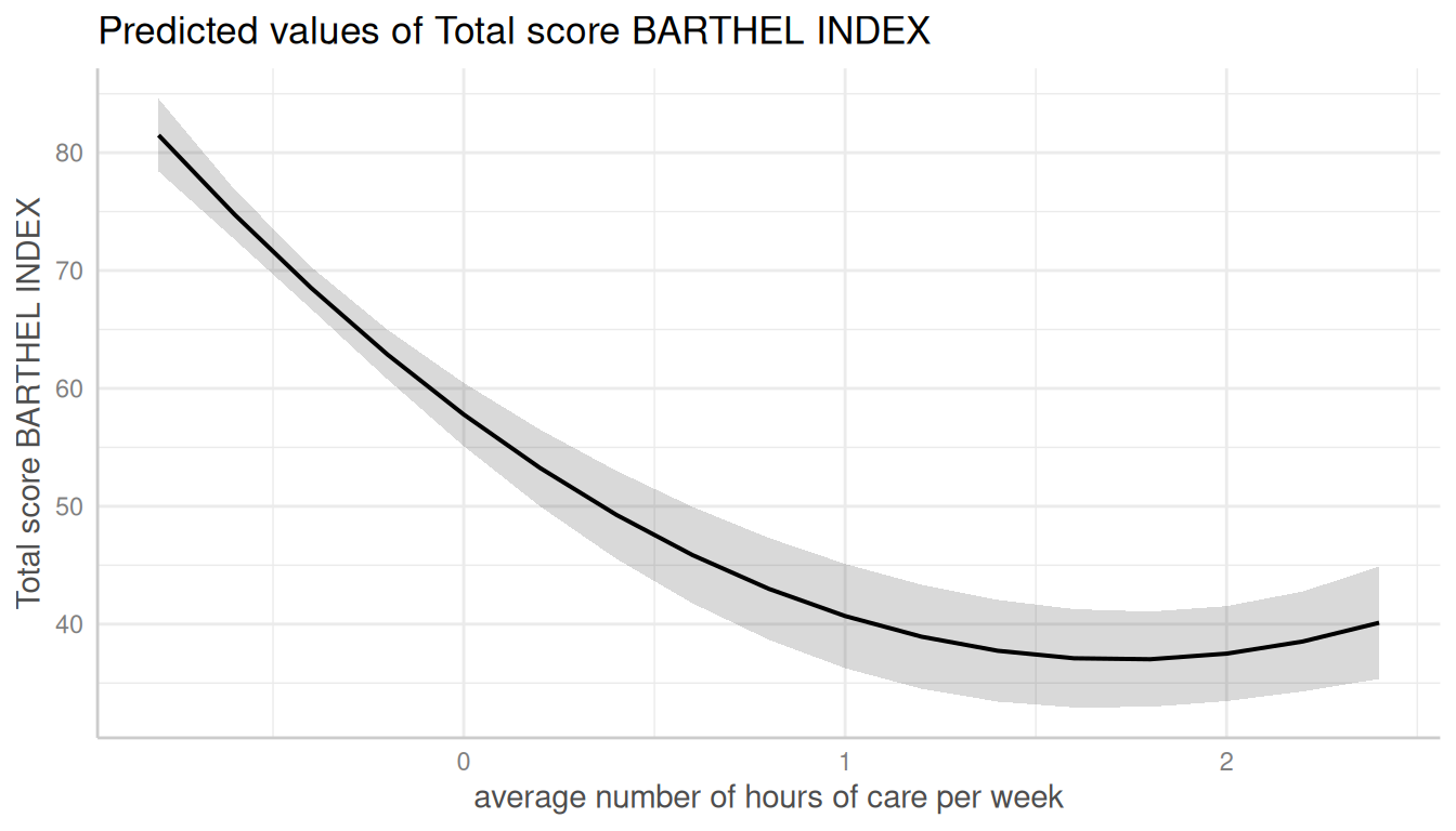

Adjusted predictions conditioned on specific values of the covariates

By default, the typical-argument determines the function that will be applied to the covariates to hold these terms at constant values. By default, this is the mean-value, but other options (like median or mode) are possible as well.

Use the condition-argument to define other values at which covariates should be held constant. condition requires a named vector, with the name indicating the covariate.

data(mtcars)
mpg_model <- lm(mpg ~ log(hp) + disp, data = mtcars)

# "disp" is hold constant at its mean
predict_response(mpg_model, "hp")
#> # Predicted values of mpg
#> 
#>  hp | Predicted |       95% CI
#> ------------------------------
#>  50 |     25.84 | 21.86, 29.82
#>  85 |     22.70 | 20.67, 24.72
#> 120 |     20.65 | 19.55, 21.76
#> 155 |     19.13 | 17.91, 20.35
#> 195 |     17.77 | 15.91, 19.64
#> 230 |     16.79 | 14.36, 19.23
#> 265 |     15.95 | 13.00, 18.91
#> 335 |     14.56 | 10.73, 18.40
#> 
#> Adjusted for:
#> * disp = 230.72

# "disp" is hold constant at value 200
predict_response(mpg_model, "hp", condition = c(disp = 200))
#> # Predicted values of mpg
#> 
#>  hp | Predicted |       95% CI
#> ------------------------------
#>  50 |     26.53 | 22.91, 30.15
#>  85 |     23.38 | 21.66, 25.11
#> 120 |     21.34 | 20.27, 22.41
#> 155 |     19.82 | 18.34, 21.30
#> 195 |     18.46 | 16.25, 20.67
#> 230 |     17.48 | 14.68, 20.28
#> 265 |     16.64 | 13.31, 19.97
#> 335 |     15.25 | 11.03, 19.47

Adjusted predictions for each level of random effects (unit-level predictions)

Adjusted predictions can also be calculated for each group level in mixed models. Simply add the name of the related random effects term to the terms-argument, and set type = "random".

In the following example, we fit a linear mixed model and first plot the population-level predictions. Please see also the dedicated vignette for mixed models for further details and examples.

library(lme4)
data(efc, package = "ggeffects")
efc$e15relat <- to_factor(efc$e15relat)
m <- lmer(neg_c_7 ~ c12hour + c160age + c161sex + (1 | e15relat), data = efc)
me <- predict_response(m, terms = "c12hour")
plot(me)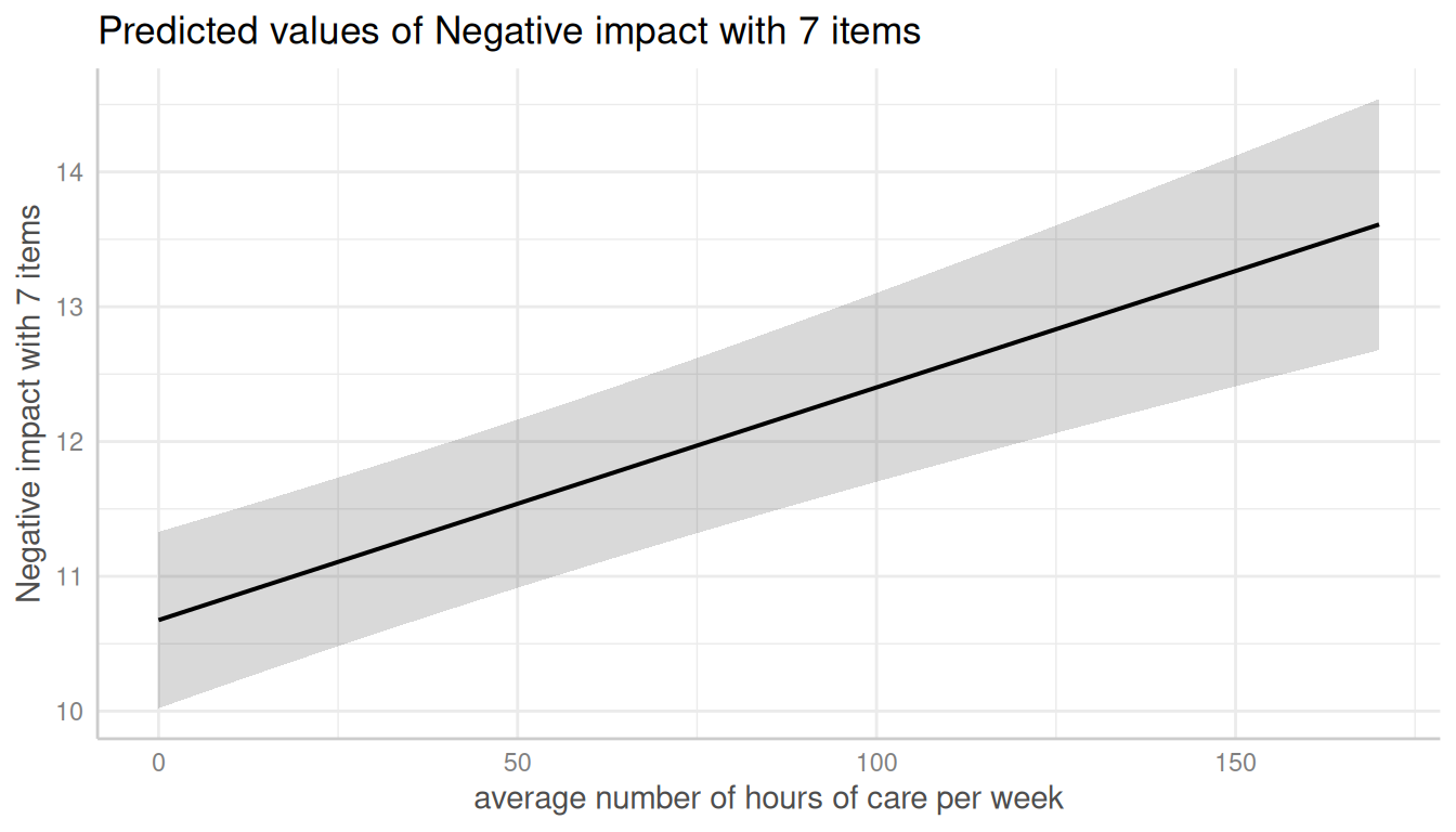

To compute adjusted predictions for each grouping level (unit-level predictions), add the related random term to the terms-argument.

me <- predict_response(m, terms = c("c12hour", "e15relat"), type = "random")
plot(me)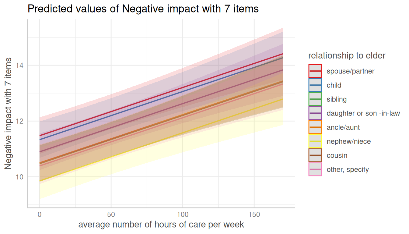

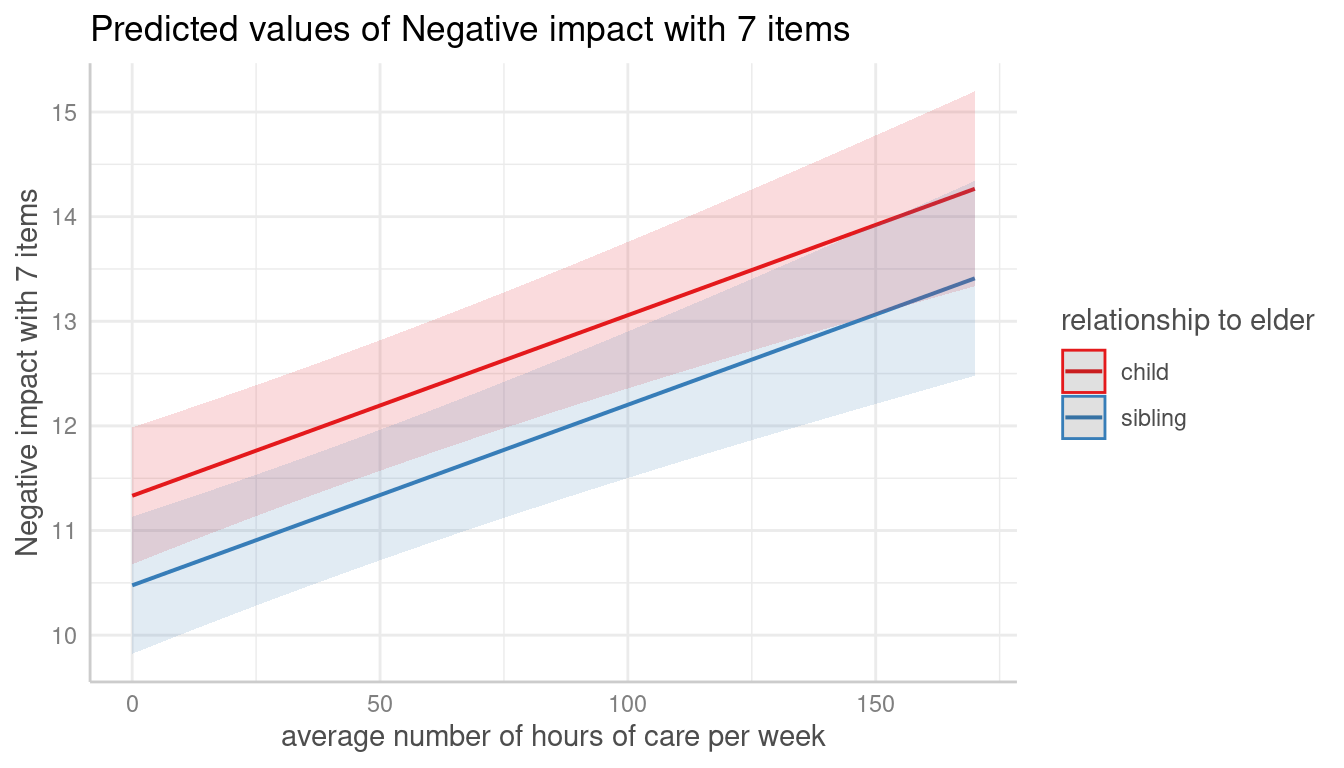
Unit-level predictions can also be calculated for specific levels only. Add the related values into brackets after the variable name in the terms-argument.

me <- predict_response(m, terms = c("c12hour", "e15relat [child,sibling]"), type = "random")
plot(me)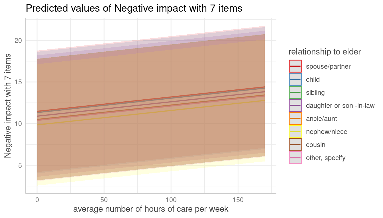

If the group factor has too many levels, you can also take a random sample of all possible levels and plot the adjusted predictions for this subsample of group levels. To do this, use term = "<groupfactor> [sample=n]".

data("sleepstudy")
m <- lmer(Reaction ~ Days + (1 + Days | Subject), data = sleepstudy)
me <- predict_response(m, terms = c("Days", "Subject [sample=8]"), type = "random")
plot(me)