Introduction: Adjusted Predictions and Marginal Effects for Random Effects Models

## Error in get(paste0(generic, ".", class), envir = get_method_env()) : 
##   object 'type_sum.accel' not found

This vignette shows how to calculate adjusted predictions for mixed models. However, for mixed models, since random effects are involved, we can calculate conditional predictions and marginal predictions. We also have to distinguish between population-level and unit-level predictions.

But one thing at a time…

Summary of most important points:

• Predictions can be made on the population-level or for each level of the grouping variable (unit-level). If unit-level predictions are requested, you need to set type="random" and specify the grouping variable(s) in the terms argument.
• Population-level predictions can be either conditional (predictions for a "typical" group) or marginal (average predictions across all groups). Set margin="empirical" for marginal predictions. You'll notice differences in predictions especially for unequal group sizes at the random effects level.
• Prediction intervals, i.e. when interval="prediction" also account for the uncertainty in the random effects.

Population-level predictions for mixed effects models

Mixed models are used to account for the dependency of observations within groups, e.g. repeated measurements within subjects, or students within schools. The dependency is modeled by random effects, i.e. mixed model at least have one grouping variable (or factor) as higher level unit.

At the lowest level, you have your fixed effects, i.e. your “independent variables” or “predictors”.

Adjusted predictions can now be calculated for specified values or levels of the focal terms, however, either for the full sample (population-level) or for each level of the grouping variable (unit-level). The latter is particularly useful when the grouping variable is of interest, e.g. when you want to compare the effect of a predictor between different groups.

To get population-level predictions, we set type = "fixed" or type = "zero_inflation" (for models with zero-inflation component).

Conditional and marginal effects/predictions

We start with the population-level predictions. Here you can either calculate the conditional or the marginal effect (see in detail also Heiss 2022). The conditional effect is the effect of a predictor in an average or typical group, while the marginal effect is the average effect of a predictor across all groups. E.g. let’s say we have countries as grouping variable and gdp (gross domestic product per capita) as predictor, then the conditional and marginal effect would be:

• conditional effect: effect of gdp in an average or typical country. To get conditional predictions, we use predict_response() or predict_response(margin = "mean_mode").

• marginal effect: average effect of gdp across all countries. To get marginal (or average) predictions, we use predict_response(margin = "empirical").

While the term “effect” referes to the strength of the relationship between a predictor and the response, “predictions” refer to the actual predicted values of the response. Thus, in the following, we will talk about conditional and marginal (or average) predictions (instead of effects).

In a balanced data set, where all groups have the same number of observations, the conditional and marginal predictions are often similar (maybe slightly different, depending on the non-focal predictors). However, in unbalanced data, the conditional and marginal predicted values can largely differ.

library(ggeffects)
library(lme4)
data(sleepstudy)

# balanced data set
m <- lmer(Reaction ~ Days + (1 + Days | Subject), data = sleepstudy)

# conditional predictions
predict_response(m, "Days [1,5,9]")
#> # Predicted values of Reaction
#> 
#> Days | Predicted |         95% CI
#> ---------------------------------
#>    1 |    261.87 | 248.48, 275.27
#>    5 |    303.74 | 284.83, 322.65
#>    9 |    345.61 | 316.74, 374.48
#> 
#> Adjusted for:
#> * Subject = 0 (population-level)

# average marginal predictions
predict_response(m, "Days [1,5,9]", margin = "empirical")
#> # Average predicted values of Reaction
#> 
#> Days | Predicted |         95% CI
#> ---------------------------------
#>    1 |    261.87 | 248.48, 275.27
#>    5 |    303.74 | 284.83, 322.65
#>    9 |    345.61 | 316.74, 374.48

# create imbalanced data set
set.seed(123)
strapped <- sleepstudy[sample.int(nrow(sleepstudy), nrow(sleepstudy), replace = TRUE), ]
m <- lmer(Reaction ~ Days + (1 + Days | Subject), data = strapped)

# conditional predictions
predict_response(m, "Days [1,5,9]")
#> # Predicted values of Reaction
#> 
#> Days | Predicted |         95% CI
#> ---------------------------------
#>    1 |    261.49 | 246.57, 276.40
#>    5 |    302.13 | 281.30, 322.97
#>    9 |    342.78 | 311.19, 374.37
#> 
#> Adjusted for:
#> * Subject = 0 (population-level)

# average marginal predictions
predict_response(m, "Days [1,5,9]", margin = "empirical")
#> # Average predicted values of Reaction
#> 
#> Days | Predicted |         95% CI
#> ---------------------------------
#>    1 |    259.04 | 244.13, 273.95
#>    5 |    300.01 | 279.17, 320.84
#>    9 |    340.97 | 309.37, 372.56

Population-level predictions and the REML argument

The conditional predictions returned by predict_response() for the default marginalization (i.e. when margin = "mean_reference" or "mean_mode") may differ…

• depending on the setting of the REML argument during model fitting;
• and depending on whether factors are included in the model or not.

library(glmmTMB)
set.seed(123)
sleepstudy$x <- as.factor(sample(1:3, nrow(sleepstudy), replace = TRUE))
# REML is FALSE
m1 <- glmmTMB(Reaction ~ Days + x + (1 + Days | Subject), data = sleepstudy, REML = FALSE)
# REML is TRUE
m2 <- glmmTMB(Reaction ~ Days + x + (1 + Days | Subject), data = sleepstudy, REML = TRUE)

# predictions when REML is FALSE
predict_response(m1, "Days [1:3]")
#> # Predicted values of Reaction
#> 
#> Days | Predicted |         95% CI
#> ---------------------------------
#>    1 |    260.22 | 245.82, 274.63
#>    2 |    270.69 | 255.77, 285.61
#>    3 |    281.16 | 265.19, 297.12
#> 
#> Adjusted for:
#> *       x = 1
#> * Subject = NA (population-level)

# predictions when REML is TRUE
predict_response(m2, "Days [1:3]")
#> # Predicted values of Reaction
#> 
#> Days | Predicted |         95% CI
#> ---------------------------------
#>    1 |    254.63 | 246.25, 263.02
#>    2 |    265.07 | 257.33, 272.81
#>    3 |    275.50 | 268.22, 282.78
#> 
#> Adjusted for:
#> *       x = 1
#> * Subject = NA (population-level)

Population-level predictions for zero-inflated mixed models

For zero-inflated mixed effects models, typically fitted with the glmmTMB or GLMMadaptive packages, predict_response() can return predicted values of the response, for the different model components:

• Conditional predictions:
  • population-level predictions, conditioned on the fixed effects (conditional or “count” model) only (type = "fixed")
  • population-level predictions, conditioned on the fixed effects and zero-inflation component (type = "zero_inflated"), returning the expected (predicted) values of the response
  • the zero-inflation probabilities (type = "zi_prob")
• Marginal predictions:
  • type = "simulate" can be used to obtain marginal predictions, averaged across all random effects groups and non-focal terms
  • marginal predictions using margin = "empirical" are also averaged across all random effects groups and non-focal terms. The major difference to type = "simulate" is that margin = "empirical" also returns counterfactual predictions.

For predict_response(margin = "empirical"), valid values for type are usually those based on the model’s predict() method. For models of class glmmTMB, these are "response", "link", "conditional", "zprob", "zlink", or "disp". However, for zero-inflated models, type = "fixed" and type = "zero_inflated" can be used as aliases (instead of "conditional" or "response").

Conditional predictions for the count model

First, we show examples for conditional predictions, which is the default marginalization method in predict_response().

library(glmmTMB)
data(Salamanders)
m <- glmmTMB(
  count ~ spp + mined + (1 | site),
  ziformula = ~ spp + mined,
  family = poisson(),
  data = Salamanders
)

Similar to mixed models without zero-inflation component, type = "fixed" returns predictions on the population-level, but for the conditional (“count”) model only.

predict_response(m, "spp")
#> # Predicted (conditional) counts of count
#> 
#> spp   | Predicted |     95% CI
#> ------------------------------
#> GP    |      0.73 | 0.42, 1.28
#> PR    |      0.42 | 0.20, 0.87
#> DM    |      0.94 | 0.56, 1.58
#> EC-A  |      0.60 | 0.33, 1.10
#> EC-L  |      1.42 | 0.85, 2.37
#> DES-L |      1.34 | 0.79, 2.26
#> DF    |      0.78 | 0.46, 1.31
#> 
#> Adjusted for:
#> * mined = yes
#> *  site = NA (population-level)

Conditional predictions for the full model

For type = "zero_inflated", results the expected values of the response, mu*(1-p). Since the zero inflation and the conditional model are working in “opposite directions”, a higher expected value for the zero inflation means a lower response, but a higher value for the conditional (“count”) model means a higher response. While it is possible to calculate predicted values with predict(..., type = "response"), standard errors and confidence intervals can not be derived directly from the predict()-function. Thus, confidence intervals for type = "zero_inflated" are based on quantiles of simulated draws from a multivariate normal distribution (see also Brooks et al. 2017, pp.391-392 for details).

predict_response(m, "spp", type = "zero_inflated")
#> # Expected counts of count
#> 
#> spp   | Predicted |     95% CI
#> ------------------------------
#> GP    |      0.20 | 0.02, 0.38
#> PR    |      0.03 | 0.00, 0.06
#> DM    |      0.32 | 0.08, 0.56
#> EC-A  |      0.07 | 0.00, 0.13
#> EC-L  |      0.42 | 0.12, 0.73
#> DES-L |      0.49 | 0.13, 0.85
#> DF    |      0.30 | 0.09, 0.51
#> 
#> Adjusted for:
#> * mined = yes
#> *  site = NA (population-level)

Marginal predictions for the full model (simulated draws)

In the above examples, we get the conditional, not the marginal predictions. E.g., predictions are conditioned on mined when it is set to "yes", and predictions refer to a typical (random effects) group. However, it is possible to obtain predicted values by simulating from the model, where predictions are based on simulate() (see Brooks et al. 2017, pp.392-393 for details). This will return expected values of the response (marginal predictions), averaged across all random effects groups and non-focal terms. To achieve this, use type = "simulate". Note that this prediction-type usually returns larger intervals, because it accounts for all model uncertainties.

predict_response(m, "spp", type = "simulate")
#> # Expected counts of count
#> 
#> spp   | Predicted |     95% CI
#> ------------------------------
#> GP    |      1.10 | 0.00, 4.31
#> PR    |      0.30 | 0.00, 2.23
#> DM    |      1.54 | 0.00, 5.49
#> EC-A  |      0.55 | 0.00, 3.11
#> EC-L  |      2.20 | 0.00, 7.35
#> DES-L |      2.26 | 0.00, 7.14
#> DF    |      1.35 | 0.00, 4.72

Marginal predictions for the full model (average predictions)

In a similar fashion, you can obtain average marginal predictions for zero-inflated mixed models with margin = "empirical". The returned values are most comparable to predict_response(type = "simulate"), because margin = "empirical" also returns expected values of the response, averaged across all random effects groups and all non-focal terms. The next example shows the average marginal predicted values of spp on the response across all sites, taking the zero-inflation component into account (i.e. type = "zero_inflated").

predict_response(m, "spp", type = "zero_inflated", margin = "empirical")
#> # Average expected counts of count
#> 
#> spp   | Predicted |     95% CI
#> ------------------------------
#> GP    |      1.08 | 0.76, 1.41
#> PR    |      0.30 | 0.13, 0.46
#> DM    |      1.52 | 1.11, 1.94
#> EC-A  |      0.54 | 0.31, 0.78
#> EC-L  |      2.17 | 1.60, 2.74
#> DES-L |      2.24 | 1.69, 2.79
#> DF    |      1.32 | 0.96, 1.68

Bias-correction for non-Gaussian models

For non-Gaussian models, predicted values are back-transformed to the response scale. However, back-transforming the population-level predictions (in mixed models, when type = "fixed") ignores the effect of the variation around the population mean, hence, the result on the original data scale is biased due to Jensen’s inequality. In this case, it can be appropriate to apply a bias-correction. This is done by setting bias_correction = TRUE. By default, insight::get_variance_residual() is used to extract the residual variance, which is used to calculate the amount of correction. Optionally, you can provide your own estimates of uncertainty, e.g. based on insight::get_variance_random(), using the sigma argument. ggeffects will warn users once per session whenever bias-correction can be appropriate.

# no bias-correction
predict_response(m, "spp")
#> You are calculating adjusted predictions on the population-level (i.e. `type = "fixed"`) for a *generalized* linear mixed model.
#>   This may produce biased estimates due to Jensen's inequality. Consider setting `bias_correction = TRUE` to correct for this bias.
#>   See also the documentation of the `bias_correction` argument.
#> # Predicted (conditional) counts of count
#> 
#> spp   | Predicted |     95% CI
#> ------------------------------
#> GP    |      0.73 | 0.42, 1.28
#> PR    |      0.42 | 0.20, 0.87
#> DM    |      0.94 | 0.56, 1.58
#> EC-A  |      0.60 | 0.33, 1.10
#> EC-L  |      1.42 | 0.85, 2.37
#> DES-L |      1.34 | 0.79, 2.26
#> DF    |      0.78 | 0.46, 1.31
#> 
#> Adjusted for:
#> * mined = yes
#> *  site = NA (population-level)

# bias-correction
predict_response(m, "spp", bias_correction = TRUE)
#> # Predicted (conditional) counts of count
#> 
#> spp   | Predicted |     95% CI
#> ------------------------------
#> GP    |      0.97 | 0.55, 1.69
#> PR    |      0.55 | 0.27, 1.15
#> DM    |      1.24 | 0.73, 2.09
#> EC-A  |      0.79 | 0.43, 1.45
#> EC-L  |      1.87 | 1.12, 3.12
#> DES-L |      1.76 | 1.04, 2.98
#> DF    |      1.02 | 0.60, 1.74
#> 
#> Adjusted for:
#> * mined = yes
#> *  site = NA (population-level)

# bias-correction, using user-defined sigma-value
predict_response(m, "spp", bias_correction = TRUE, sigma = insight::get_sigma(m))
#> # Predicted (conditional) counts of count
#> 
#> spp   | Predicted |     95% CI
#> ------------------------------
#> GP    |      1.10 | 0.63, 1.92
#> PR    |      0.63 | 0.30, 1.30
#> DM    |      1.41 | 0.83, 2.38
#> EC-A  |      0.90 | 0.49, 1.65
#> EC-L  |      2.13 | 1.27, 3.55
#> DES-L |      2.01 | 1.19, 3.39
#> DF    |      1.16 | 0.69, 1.97
#> 
#> Adjusted for:
#> * mined = yes
#> *  site = NA (population-level)

Unit-level predictions (predictions for each level of random effects)

Adjusted predictions can also be calculated for each group level (unit-level) in mixed models. Simply add the name of the related random effects term to the terms-argument, and set type = "random". For predict_response(margin = "empirical"), you don’t need to set type = "random".

In the following example, we fit a linear mixed model and first simply plot the adjusted predictions at the population-level.

library(sjlabelled)
data(efc)
efc$e15relat <- as_label(efc$e15relat)
m <- lmer(neg_c_7 ~ c12hour + c160age + c161sex + (1 | e15relat), data = efc)
me <- predict_response(m, terms = "c12hour")
plot(me)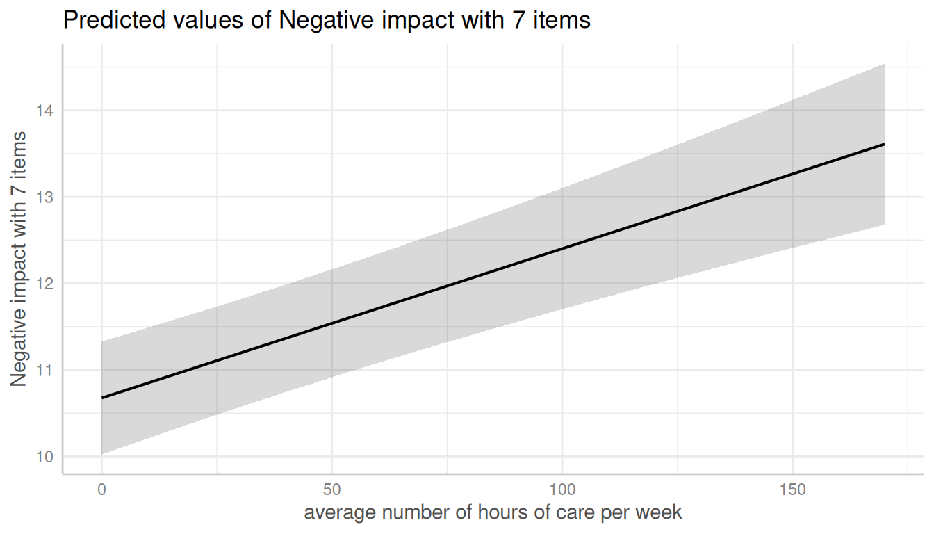

To compute adjusted predictions for each grouping level (unit-level), add the related random effects term to the terms-argument. In this case, predictions are calculated for each level of the specified random effects term.

me <- predict_response(m, terms = c("c12hour", "e15relat"), type = "random")
plot(me, show_ci = FALSE)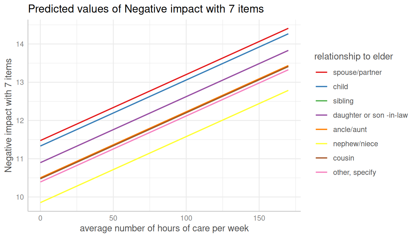

Since average marginal predictions already consider random effects by averaging over the groups, the type-argument is not needed when margin = "empirical" is set.

me <- predict_response(m, terms = c("c12hour", "e15relat"), margin = "empirical")
plot(me, show_ci = FALSE)

Adjusted predictions can also be calculated for specific unit-levels only. Add the related values into brackets after the variable name in the terms-argument.

me <- predict_response(m, terms = c("c12hour", "e15relat [child,sibling]"), type = "random")
plot(me, show_ci = FALSE)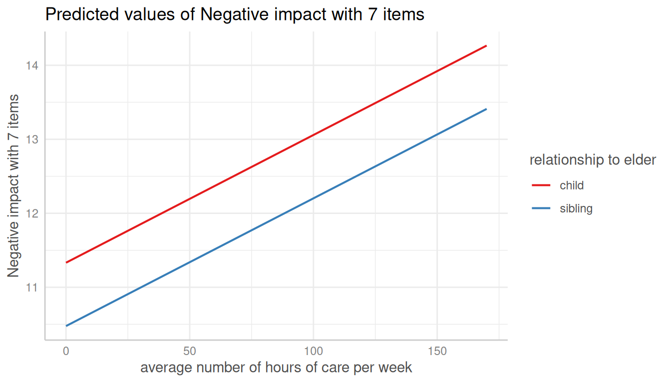

The complex plot in this scenario would be a term (c12hour) at certain values of two other terms (c161sex, c160age) for specific unit-levels of random effects (e15relat), so we have four variables in the terms-argument.

me <- predict_response(
  m,
  terms = c("c12hour", "c161sex", "c160age", "e15relat [child,sibling]"),
  type = "random"
)
plot(me)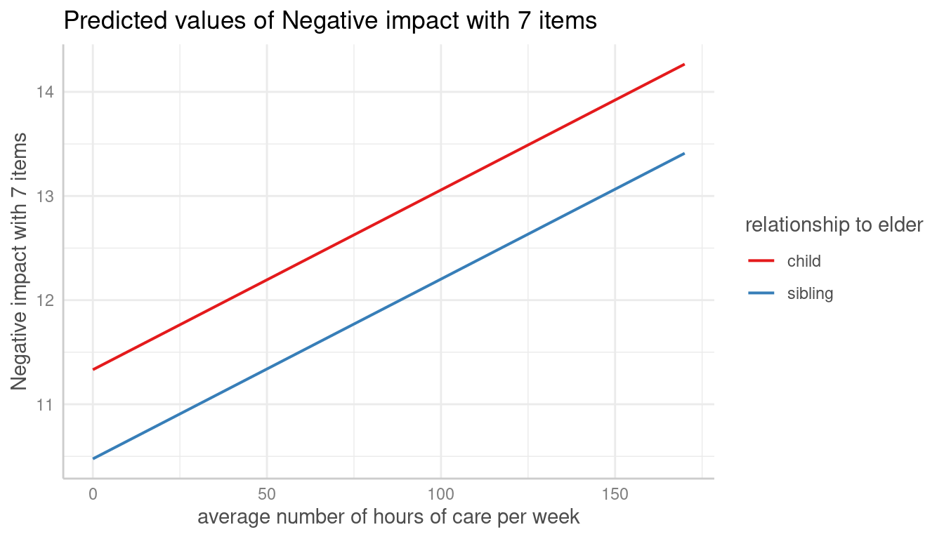

If the group factor has too many levels, you can also take a random sample of all possible levels and plot the adjusted predictions for this subsample of unit-levels. To do this, use term = "<groupfactor> [sample=n]".

set.seed(123)
m <- lmer(Reaction ~ Days + (1 + Days | Subject), data = sleepstudy)
me <- predict_response(m, terms = c("Days", "Subject [sample=7]"), type = "random")
plot(me)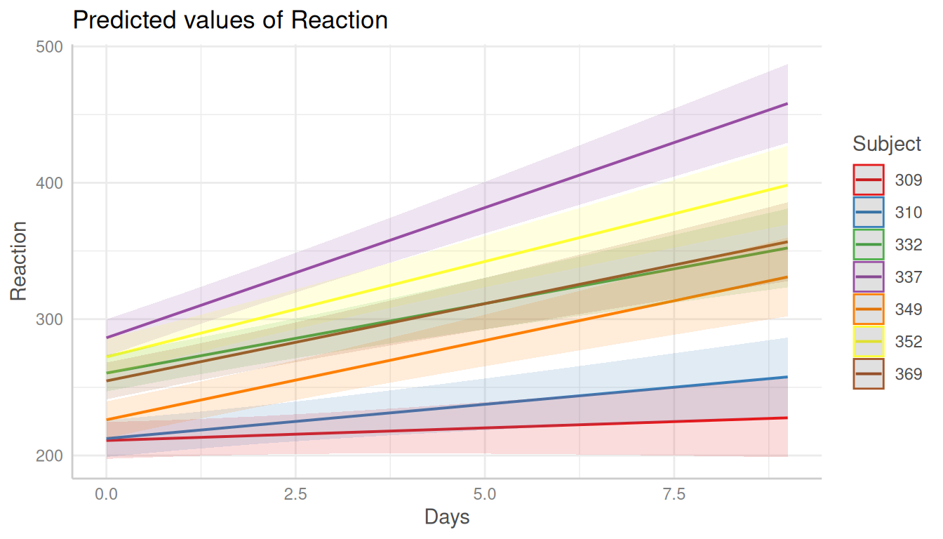

You can also add the observed data points for each group using show_data = TRUE.

plot(me, show_data = TRUE, show_ci = FALSE)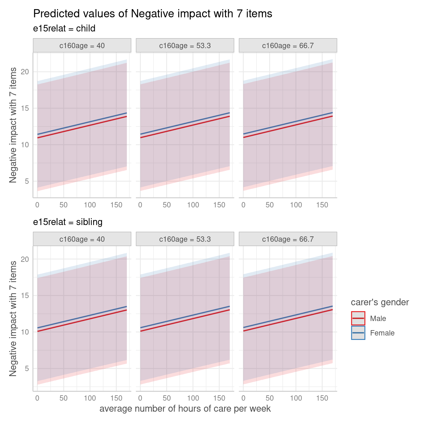

Population-level predictions for gam and glmer models

The output of predict_response() indicates that the grouping variable of the random effects is set to “population level” (adjustment), e.g. in case of lme4, following is printed:

Adjusted for: * Subject = 0 (population-level)

A comparable model fitted with mgcv::gam() would print a different message:

Adjusted for: * Subject = 308

The reason is because the correctly printed information about adjustment for random effects is based on insight::find_random(), which returns NULL for gams with random effects defined via s(..., bs = "re"). However, predictions are still correct, when population-level predictions are requested. Here’s an example:

data("sleepstudy", package = "lme4")
# mixed model with lme4
m_lmer <- lme4::lmer(Reaction ~ poly(Days, 2) + (1 | Subject),
  data = sleepstudy
)
# equivalent model, random effects are defined via s(..., bs = "re")
m_gam <- mgcv::gam(Reaction ~ poly(Days, 2) + s(Subject, bs = "re"),
  family = gaussian(), data = sleepstudy, method = "ML"
)

# predictions are identical
predict_response(m_gam, terms = "Days", exclude = "s(Subject)", newdata.guaranteed = TRUE)
#> # Predicted values of Reaction
#> 
#> Days | Predicted |         95% CI
#> ---------------------------------
#>    0 |    255.45 | 235.12, 275.78
#>    1 |    263.22 | 244.71, 281.73
#>    2 |    271.67 | 253.70, 289.63
#>    3 |    280.78 | 262.75, 298.82
#>    5 |    301.05 | 282.84, 319.25
#>    6 |    312.19 | 294.15, 330.22
#>    7 |    324.00 | 306.03, 341.97
#>    9 |    349.65 | 329.33, 369.98
#> 
#> Adjusted for:
#> * Subject = 308

predict_response(m_lmer, terms = "Days")
#> # Predicted values of Reaction
#> 
#> Days | Predicted |         95% CI
#> ---------------------------------
#>    0 |    255.45 | 234.79, 276.10
#>    1 |    263.22 | 244.35, 282.09
#>    2 |    271.67 | 253.33, 290.00
#>    3 |    280.78 | 262.38, 299.19
#>    5 |    301.05 | 282.48, 319.61
#>    6 |    312.19 | 293.78, 330.59
#>    7 |    324.00 | 305.66, 342.34
#>    9 |    349.65 | 329.00, 370.31
#> 
#> Adjusted for:
#> * Subject = 0 (population-level)

References

Brooks ME, Kristensen K, Benthem KJ van, Magnusson A, Berg CW, Nielsen A, et al. glmmTMB Balances Speed and Flexibility Among Packages for Zero-inflated Generalized Linear Mixed Modeling. The R Journal. 2017;9: 378–400.

Heiss, A. (2022, November 29). Marginal and conditional effects for GLMMs with {marginaleffects}. Andrew Heiss’s Blog. (doi: 10.59350/xwnfm-x1827)

Johnson PC. 2014. Extension of Nakagawa & Schielzeth’s R2GLMM to random slopes models. Methods Ecol Evol, 5: 944-946. (doi: 10.1111/2041-210X.12225)