Case Study: (Cluster) Robust Standard Errors

This vignette demonstrate how to compute confidence intervals based on (cluster) robust variance-covariance matrices for standard errors.

First, we load the required packages and create a sample data set with a binomial and continuous variable as predictor as well as a group factor.

library(ggeffects)
set.seed(123)

# example taken from "?clubSandwich::vcovCR"
m <- 8
cluster <- factor(rep(LETTERS[1:m], 3 + rpois(m, 5)))
n <- length(cluster)
X <- matrix(rnorm(3 * n), n, 3)
nu <- rnorm(m)[cluster]
e <- rnorm(n)
y <- X %*% c(0.4, 0.3, -0.3) + nu + e
dat <- data.frame(y, X, cluster, row = 1:n)

# fit linear model
model <- lm(y ~ X1 + X2 + X3, data = dat)

Predictions with normal standard errors

In this example, we use the normal standard errors, as returned by predict(), to compute confidence intervals.

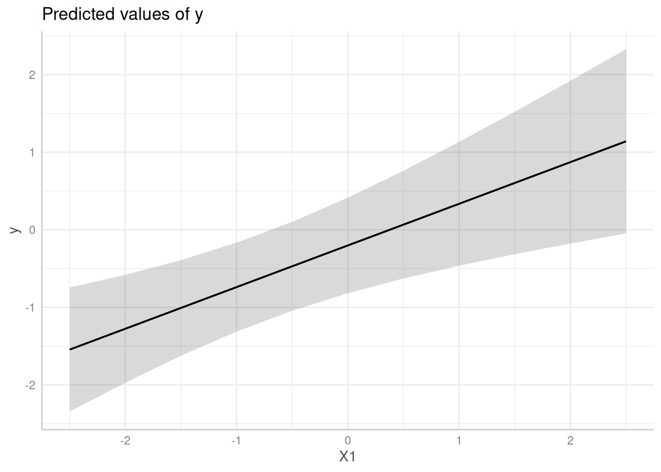
predict_response(model, "X1")
#> # Predicted values of y
#> 
#>    X1 | Predicted |       95% CI
#> --------------------------------
#> -2.50 |     -1.54 | -2.42, -0.67
#> -2.00 |     -1.28 | -2.00, -0.55
#> -1.00 |     -0.74 | -1.19, -0.29
#> -0.50 |     -0.47 | -0.81, -0.13
#>  0.00 |     -0.20 | -0.50,  0.10
#>  0.50 |      0.07 | -0.27,  0.41
#>  1.00 |      0.34 | -0.10,  0.78
#>  2.50 |      1.14 |  0.28,  2.01
#> 
#> Adjusted for:
#> * X2 = -0.08
#> * X3 =  0.09
#> 
#> Not all rows are shown in the output. Use `print(..., n = Inf)` to show
#>   all rows.

me <- predict_response(model, "X1")
plot(me)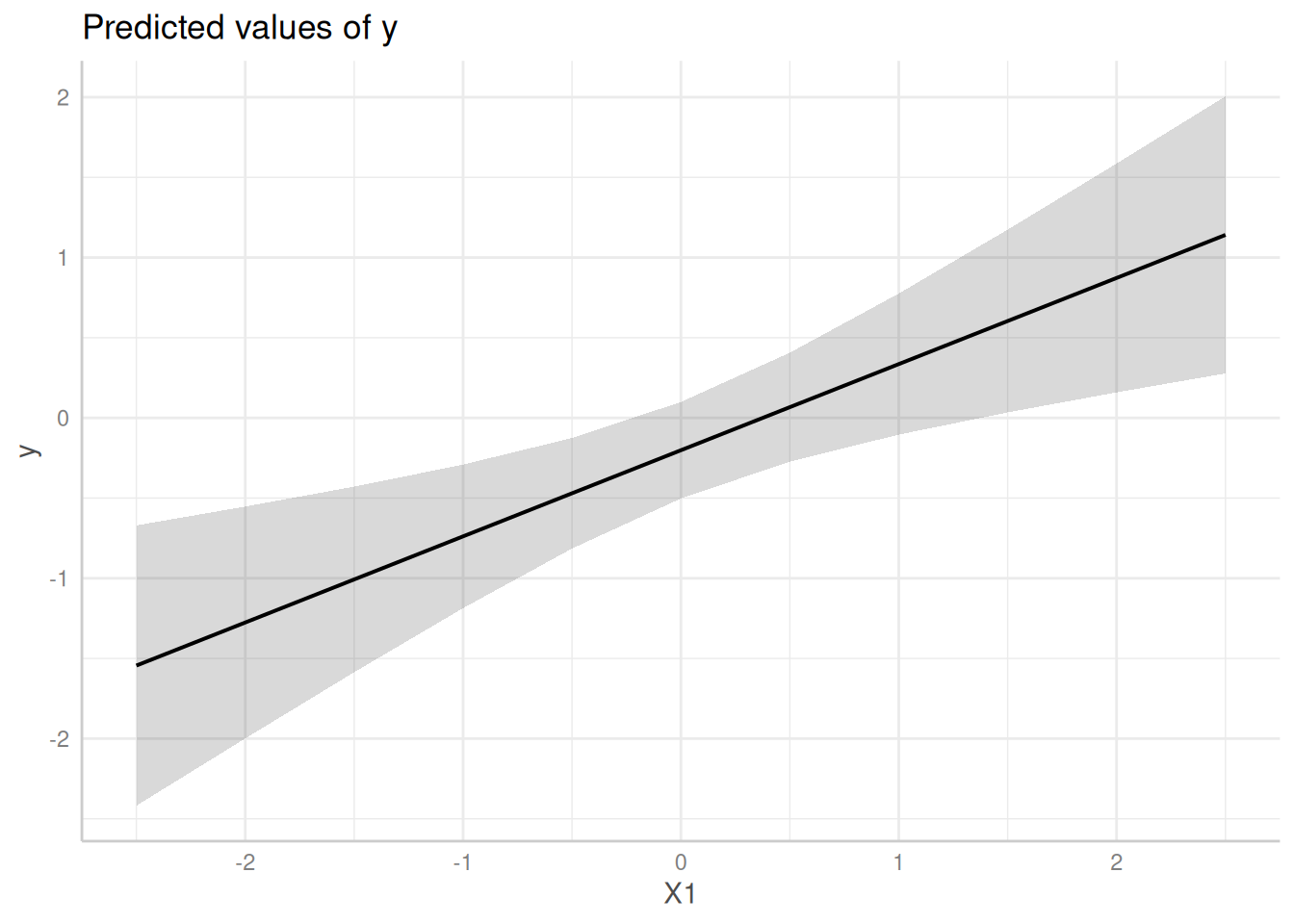

Predictions with HC-estimated standard errors

Now, we use sandwich::vcovHC() to estimate heteroskedasticity-consistent standard errors. To do so, first the function name, vcovHC(), must be supplied to the vcov_fun-argument. sandwich::vcovHC(), in turn, has different types of estimation. This must be specified in vcov_type. As a shortcut, the estimation type can be directly passed to vcov_fun, however, this would only call sandwich::vcovHC().

# shorter: predict_response(model, "X1", vcov_fun = "HC0"). This is equivalent to the following:
predict_response(model, "X1", vcov_fun = "vcovHC", vcov_type = "HC0")
#> # Predicted values of y
#> 
#>    X1 | Predicted |       95% CI
#> --------------------------------
#> -2.50 |     -1.54 | -2.41, -0.68
#> -2.00 |     -1.28 | -1.98, -0.57
#> -1.00 |     -0.74 | -1.14, -0.34
#> -0.50 |     -0.47 | -0.77, -0.17
#>  0.00 |     -0.20 | -0.49,  0.09
#>  0.50 |      0.07 | -0.31,  0.44
#>  1.00 |      0.34 | -0.17,  0.84
#>  2.50 |      1.14 |  0.15,  2.14
#> 
#> Adjusted for:
#> * X2 = -0.08
#> * X3 =  0.09
#> 
#> Not all rows are shown in the output. Use `print(..., n = Inf)` to show
#>   all rows.

me <- predict_response(model, "X1", vcov_fun = "vcovHC", vcov_type = "HC0")
plot(me)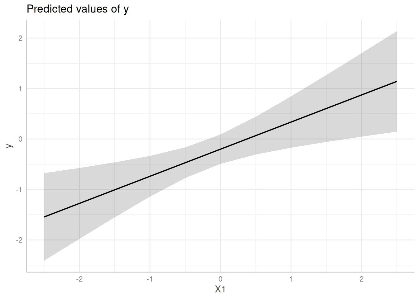

Passing a function to vcov_fun

Instead of character strings, the vcov_fun argument also accepts a function that returns a variance-covariance matrix. Further arguments that need to be passed to that functions should be provided as list to the vcov_args argument. Thus, we can rewrite the above code-chunk in the following way:

predict_response(
  model,
  "X1",
  vcov_fun = sandwich::vcovHC,
  vcov_args = list(type = "HC0")
)
#> # Predicted values of y
#> 
#>    X1 | Predicted |       95% CI
#> --------------------------------
#> -2.50 |     -1.54 | -2.41, -0.68
#> -2.00 |     -1.28 | -1.98, -0.57
#> -1.00 |     -0.74 | -1.14, -0.34
#> -0.50 |     -0.47 | -0.77, -0.17
#>  0.00 |     -0.20 | -0.49,  0.09
#>  0.50 |      0.07 | -0.31,  0.44
#>  1.00 |      0.34 | -0.17,  0.84
#>  2.50 |      1.14 |  0.15,  2.14
#> 
#> Adjusted for:
#> * X2 = -0.08
#> * X3 =  0.09
#> 
#> Not all rows are shown in the output. Use `print(..., n = Inf)` to show
#>   all rows.

Predictions with cluster-robust standard errors

The last example shows how to define cluster-robust standard errors. These are based on clubSandwich::vcovCR(). Thus, vcov_fun = "vcovCR" is always required when estimating cluster robust standard errors. clubSandwich::vcovCR() has also different estimation types, which must be specified in vcov_type. Furthermore, clubSandwich::vcovCR() requires the cluster-argument, which must be specified in vcov_args:

predict_response(
  model, "X1", vcov_fun = "vcovCR", vcov_type = "CR0",
  vcov_args = list(cluster = dat$cluster)
)
#> # Predicted values of y
#> 
#>    X1 | Predicted |       95% CI
#> --------------------------------
#> -2.50 |     -1.54 | -2.34, -0.75
#> -2.00 |     -1.28 | -1.97, -0.58
#> -1.00 |     -0.74 | -1.31, -0.17
#> -0.50 |     -0.47 | -1.04,  0.10
#>  0.00 |     -0.20 | -0.82,  0.41
#>  0.50 |      0.07 | -0.63,  0.76
#>  1.00 |      0.34 | -0.46,  1.13
#>  2.50 |      1.14 | -0.05,  2.33
#> 
#> Adjusted for:
#> * X2 = -0.08
#> * X3 =  0.09
#> 
#> Not all rows are shown in the output. Use `print(..., n = Inf)` to show
#>   all rows.

me <- predict_response(
  model, "X1", vcov_fun = "vcovCR", vcov_type = "CR0",
  vcov_args = list(cluster = dat$cluster)
)
plot(me)