Technical Details: Difference Between Marginalization Methods: The `margin` Argument • ggeffects

## Error in get(paste0(generic, ".", class), envir = get_method_env()) : 
##   object 'type_sum.accel' not found

predict_response() computes marginal means or predicted values for all possible levels or values from specified model’s predictors (focal terms). These effects are “marginalized” (or “averaged”) over the values or levels of remaining predictors (the non-focal terms). The margin argument specifies the method of marginalization. The following methods are available:

"mean_reference": non-focal predictors are set to their mean (numeric variables), reference level (factors), or “most common” value (mode) in case of character vectors. Technically, a data grid is constructed, roughly comparable to expand.grid() on all unique combinations of model.frame(model)[, terms]. This data grid (see data_grid()) is used for the newdata argument of predict(). All remaining covariates not specified in terms are held constant: Numeric values are set to the mean, integer values are set to their median, factors are set to their reference level and character vectors to their mode (most common element).
"mean_mode": non-focal predictors are set to their mean (numeric variables) or mode (factors, or “most common” value in case of character vectors).
"marginalmeans": non-focal predictors are set to their mean (numeric variables) or marginalized over the levels or “values” for factors and character vectors. Marginalizing over the factor levels of non-focal terms computes a kind of “weighted average” for the values at which these terms are hold constant.
"empirical" (or "counterfactual"): non-focal predictors are marginalized over the observations in your sample, for counterfactual predictions. Technically, predicted values for each observation in the data are calculated multiple times (the data is duplicated once for all unique values of the focal terms), each time fixing one unique value or level of the focal terms and then takes the average of these predicted values (aggregated/grouped by the focal terms).

That means:

For models without categorical predictors, results are usually identical, no matter which margin option is selected (except some slight differences in the associated confidence intervals, which are, however, negligible).
When all categorical predictors are specified in terms and further (non-focal) terms are only numeric, results are usually identical, as well.

In the general introduction, the margin argument is discussed more in detail, providing hints on when to use which method. Here, we will provide a more technical explanation of the differences between the methods.

library(ggeffects)
data(efc, package = "ggeffects")
fit <- lm(barthtot ~ c12hour + neg_c_7, data = efc)

# we add margin = "mean_reference" to show that it is the default
predict_response(fit, "c12hour [0,50,100,150]", margin = "mean_reference")
#> # Predicted values of Total score BARTHEL INDEX
#> 
#> c12hour | Predicted |       95% CI
#> ----------------------------------
#>       0 |     75.07 | 72.96, 77.19
#>      50 |     62.78 | 61.16, 64.40
#>     100 |     50.48 | 48.00, 52.97
#>     150 |     38.19 | 34.30, 42.08
#> 
#> Adjusted for:
#> * neg_c_7 = 11.83

predict_response(fit, "c12hour [0,50,100,150]", margin = "marginalmeans")
#> # Predicted values of Total score BARTHEL INDEX
#> 
#> c12hour | Predicted |       95% CI
#> ----------------------------------
#>       0 |     75.07 | 72.96, 77.19
#>      50 |     62.78 | 61.16, 64.40
#>     100 |     50.48 | 48.00, 52.97
#>     150 |     38.19 | 34.30, 42.08
#> 
#> Adjusted for:
#> * neg_c_7 = 11.83

As can be seen, the continuous predictor neg_c_7 is held constant at its mean value, 11.83. For categorical predictors, margin = "mean_reference" (the default, and thus not specified in the above example) and margin = "marginalmeans" behave differently. While "mean_reference" uses the reference level of each categorical predictor to hold it constant, "marginalmeans" averages over the proportions of the categories of factors.

library(datawizard)
data(efc, package = "ggeffects")
efc$e42dep <- to_factor(efc$e42dep)
# we add categorical predictors to our model
fit <- lm(barthtot ~ c12hour + neg_c_7 + e42dep, data = efc)

predict_response(fit, "c12hour [0,50,100,150]", margin = "mean_reference")
#> # Predicted values of Total score BARTHEL INDEX
#> 
#> c12hour | Predicted |       95% CI
#> ----------------------------------
#>       0 |     92.74 | 88.48, 97.01
#>      50 |     89.18 | 84.82, 93.54
#>     100 |     85.61 | 80.79, 90.42
#>     150 |     82.04 | 76.49, 87.59
#> 
#> Adjusted for:
#> * neg_c_7 =       11.83
#> *  e42dep = independent

predict_response(fit, "c12hour [0,50,100,150]", margin = "marginalmeans")
#> # Predicted values of Total score BARTHEL INDEX
#> 
#> c12hour | Predicted |       95% CI
#> ----------------------------------
#>       0 |     73.51 | 71.85, 75.18
#>      50 |     69.95 | 68.51, 71.38
#>     100 |     66.38 | 64.19, 68.56
#>     150 |     62.81 | 59.51, 66.10
#> 
#> Adjusted for:
#> * neg_c_7 = 11.83

In this case, one would obtain the same results for "mean_reference" and "marginalmeans" again, if condition is used to define specific levels at which variables, in our case the factor e42dep, should be held constant.

predict_response(fit, "c12hour [0,50,100,150]", margin = "mean_reference")
#> # Predicted values of Total score BARTHEL INDEX
#> 
#> c12hour | Predicted |       95% CI
#> ----------------------------------
#>       0 |     92.74 | 88.48, 97.01
#>      50 |     89.18 | 84.82, 93.54
#>     100 |     85.61 | 80.79, 90.42
#>     150 |     82.04 | 76.49, 87.59
#> 
#> Adjusted for:
#> * neg_c_7 =       11.83
#> *  e42dep = independent

predict_response(
  fit,
  "c12hour [0,50,100,150]",
  margin = "marginalmeans",
  condition = c(e42dep = "independent")
)
#> # Predicted values of Total score BARTHEL INDEX
#> 
#> c12hour | Predicted |       95% CI
#> ----------------------------------
#>       0 |     92.74 | 88.48, 97.01
#>      50 |     89.18 | 84.82, 93.54
#>     100 |     85.61 | 80.79, 90.42
#>     150 |     82.04 | 76.49, 87.59
#> 
#> Adjusted for:
#> * neg_c_7 = 11.83

Another option is to use predict_response(margin = "empirical") to compute “counterfactual” adjusted predictions. This function is a wrapper for the avg_predictions()-method from the marginaleffects-package. The major difference to margin = "marginalmeans" is that estimated marginal means, as computed by "marginalmeans", are a special case of predictions, made on a perfectly balanced grid of categorical predictors, with numeric predictors held at their means, and marginalized with respect to some focal variables.

predict_response(margin = "empirical"), in turn, calculates predicted values for each observation in the data multiple times, each time fixing the unique values or levels of the focal terms to one specific value and then takes the average of these predicted values (aggregated/grouped by the focal terms) - or in other words: the whole dataset is duplicated once for every unique value of the focal terms, makes predictions for each observation of the new dataset and take the average of all predictions (grouped by focal terms). This is also called “counterfactual” predictions.

predict_response(fit, "c12hour", margin = "empirical")
#> # Average predicted values of Total score BARTHEL INDEX
#> 
#> c12hour | Predicted |       95% CI
#> ----------------------------------
#>       0 |     67.73 | 66.15, 69.31
#>      20 |     66.30 | 65.03, 67.57
#>      45 |     64.52 | 63.38, 65.66
#>      65 |     63.09 | 61.81, 64.37
#>      85 |     61.66 | 60.07, 63.25
#>     105 |     60.23 | 58.24, 62.23
#>     125 |     58.81 | 56.37, 61.25
#>     170 |     55.59 | 52.08, 59.11

To explain how margin = "empirical" works, let’s look at following example, where we compute the average predicted values and the estimated marginal means manually. The confidence intervals for the manually calculated means differ from those of predict_response(), however, the predicted and manually calculated mean values are identical.

data(iris)
set.seed(123)
iris$x <- as.factor(sample(1:4, nrow(iris), replace = TRUE, prob = c(0.1, 0.2, 0.3, 0.4)))
m <- lm(Sepal.Width ~ Species + x, data = iris)

# average predicted values
predict_response(m, "Species", margin = "empirical")
#> # Average predicted values of Sepal.Width
#> 
#> Species    | Predicted |     95% CI
#> -----------------------------------
#> setosa     |      3.43 | 3.34, 3.52
#> versicolor |      2.77 | 2.67, 2.86
#> virginica  |      2.97 | 2.88, 3.07

# replicate the dataset for each level of "Species", i.e. 3 times
d <- do.call(rbind, replicate(3, iris, simplify = FALSE))
# for each data set, we set our focal term to one of the three levels
d$Species <- as.factor(rep(levels(iris$Species), each = 150))
# we calculate predicted values for each "dataset", i.e. we predict our outcome
# for observations, for all levels of "Species"
d$predicted <- predict(m, newdata = d)
# now we compute the average predicted values by levels of "Species", where
# non-focal terms are weighted proportional to their occurence in the data
datawizard::means_by_group(d, "predicted", "Species")
#> # Mean of predicted by Species
#> 
#> Category   | Mean |   N |   SD |       95% CI |      p
#> ------------------------------------------------------
#> setosa     | 3.43 | 150 | 0.06 | [3.42, 3.44] | < .001
#> versicolor | 2.77 | 150 | 0.06 | [2.76, 2.78] | < .001
#> virginica  | 2.97 | 150 | 0.06 | [2.96, 2.98] | < .001
#> Total      | 3.06 | 450 | 0.28 |              |       
#> 
#> Anova: R2=0.951; adj.R2=0.951; F=4320.998; p<.001

# estimated marginal means, in turn, differ from the above, because they are
# averaged across balanced reference grids for all focal terms, thereby non-focal
# are hold constant at an (equally) "weighted average".

# estimated marginal means, from `ggemmeans()`
predict_response(m, "Species", margin = "marginalmeans")
#> # Predicted values of Sepal.Width
#> 
#> Species    | Predicted |     95% CI
#> -----------------------------------
#> setosa     |      3.45 | 3.35, 3.54
#> versicolor |      2.78 | 2.68, 2.89
#> virginica  |      2.99 | 2.89, 3.09

d <- rbind(
  data_grid(m, "Species", condition = c(x = "1")),
  data_grid(m, "Species", condition = c(x = "2")),
  data_grid(m, "Species", condition = c(x = "3")),
  data_grid(m, "Species", condition = c(x = "4"))
)
d$predicted <- predict(m, newdata = d)
# means calculated manually
datawizard::means_by_group(d, "predicted", "Species")
#> # Mean of predicted by Species
#> 
#> Category   | Mean |  N |   SD |       95% CI |      p
#> -----------------------------------------------------
#> setosa     | 3.45 |  4 | 0.07 | [3.36, 3.53] | < .001
#> versicolor | 2.78 |  4 | 0.07 | [2.70, 2.87] | < .001
#> virginica  | 2.99 |  4 | 0.07 | [2.91, 3.07] | 0.019 
#> Total      | 3.07 | 12 | 0.30 |              |       
#> 
#> Anova: R2=0.952; adj.R2=0.941; F=88.566; p<.001

But when should I use which margin option?

When you are interested in the strength of association, it usually doesn’t matter. as you can see in the plots below. The slope of our focal term, c12hour, is the same for all four plots:

library(see)
predicted_1 <- predict_response(fit, terms = "c12hour")
predicted_2 <- predict_response(fit, terms = "c12hour", margin = "marginalmeans")
predicted_3 <- predict_response(fit, terms = "c12hour", margin = "marginalmeans", condition = c(e42dep = "independent"))
predicted_4 <- predict_response(fit, terms = "c12hour", margin = "empirical")

p1 <- plot(predicted_1, show_ci = FALSE, show_title = FALSE, show_x_title = FALSE, show_y_title = FALSE)
p2 <- plot(predicted_2, show_ci = FALSE, show_title = FALSE, show_x_title = FALSE, show_y_title = FALSE)
p3 <- plot(predicted_3, show_ci = FALSE, show_title = FALSE, show_x_title = FALSE, show_y_title = FALSE)
p4 <- plot(predicted_4, show_ci = FALSE, show_title = FALSE, show_x_title = FALSE, show_y_title = FALSE)

plots(p1, p2, p3, p4, n_rows = 2)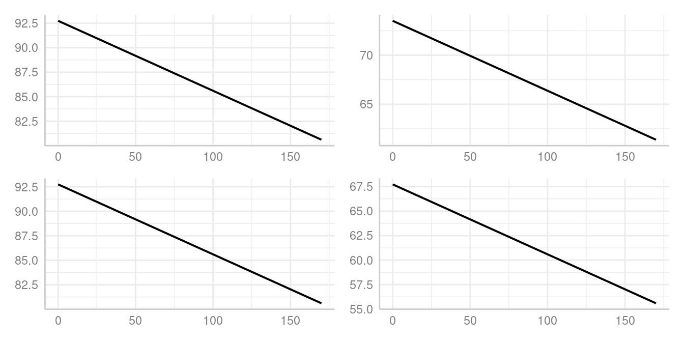

However, the predicted outcome varies. The general introduction discusses the margin argument more in detail, but a few hints on when to use which method are following:

Predictions based on "mean_reference" and "mean_mode" represent a rather “theoretical” view on your data, which does not necessarily exactly reflect the characteristics of your sample. It helps answer the question, “What is the predicted value of the response at meaningful values or levels of my focal terms for a ‘typical’ observation in my data?”, where ‘typical’ refers to certain characteristics of the remaining predictors.
"marginalmeans" comes closer to the sample, because it takes all possible values and levels of your non-focal predictors into account. It would answer thr question, “What is the predicted value of the response at meaningful values or levels of my focal terms for an ‘average’ observation in my data?”. It refers to randomly picking a subject of your sample and the result you get on average.
"empirical"is probably the most “realistic” approach, insofar as the results can also be transferred to other contexts. It answers the question, “What is the predicted value of the response at meaningful values or levels of my focal terms for the ‘average’ observation in the population?”. It does not only refer to the actual data in your sample, but also “what would be if” we had more data, or if we had data from a different population. This is where “counterfactual” refers to.

What is the most apparent difference from margin = "empirical" to the other options?

The most apparent difference from margin = "empirical" compared to the other methods occurs when you have categorical co-variates (non-focal terms) with unequally distributed levels. margin = "marginalmeans" will “average” over the levels of non-focal factors, while margin = "empirical" will average over the observations in your sample.

Let’s show this with a very simple example:

data(iris)
set.seed(123)
# create an unequal distributed factor, used as non-focal term
iris$x <- as.factor(sample(1:4, nrow(iris), replace = TRUE, prob = c(0.1, 0.2, 0.3, 0.4)))
m <- lm(Sepal.Width ~ Species + x, data = iris)

# predicted values, conditioned on x = 1
predict_response(m, "Species")
#> # Predicted values of Sepal.Width
#> 
#> Species    | Predicted |     95% CI
#> -----------------------------------
#> setosa     |      3.50 | 3.30, 3.69
#> versicolor |      2.84 | 2.63, 3.04
#> virginica  |      3.04 | 2.85, 3.23
#> 
#> Adjusted for:
#> * x = 1

# predicted values, conditioned on weighted average of x
predict_response(m, "Species", margin = "marginalmeans")
#> # Predicted values of Sepal.Width
#> 
#> Species    | Predicted |     95% CI
#> -----------------------------------
#> setosa     |      3.45 | 3.35, 3.54
#> versicolor |      2.78 | 2.68, 2.89
#> virginica  |      2.99 | 2.89, 3.09

# average predicted values, averaged over the sample and aggregated by "Species"
predict_response(m, "Species", margin = "empirical")
#> # Average predicted values of Sepal.Width
#> 
#> Species    | Predicted |     95% CI
#> -----------------------------------
#> setosa     |      3.43 | 3.34, 3.52
#> versicolor |      2.77 | 2.67, 2.86
#> virginica  |      2.97 | 2.88, 3.07

Finally, the weighting for margin = "marginalmeans" can be changed using the weights argument (for details, see ?emmeans::emmeans), which returns results that are more similar to margin = "empirical".

# the default is an equally weighted average; "proportional" weights in
# proportion to the  frequencies of factor combinations
predict_response(m, "Species", margin = "marginalmeans", weights = "proportional")
#> # Predicted values of Sepal.Width
#> 
#> Species    | Predicted |     95% CI
#> -----------------------------------
#> setosa     |      3.43 | 3.34, 3.52
#> versicolor |      2.77 | 2.67, 2.86
#> virginica  |      2.97 | 2.88, 3.07