Get titles and labels from data

Get variable and value labels from ggeffects-objects. predict_response() saves information on variable names and value labels as additional attributes in the returned data frame. This is especially helpful for labelled data (see sjlabelled), since these labels can be used to set axis labels and titles.

Usage

get_title(x, case = NULL)

get_x_title(x, case = NULL)

get_y_title(x, case = NULL)

get_legend_title(x, case = NULL)

get_legend_labels(x, case = NULL)

get_x_labels(x, case = NULL)

get_complete_df(x, case = NULL)

Arguments

x

An object of class ggeffects, as returned by any ggeffects-function; for get_complete_df(), must be a list of ggeffects-objects.

case

Desired target case. Labels will automatically converted into the specified character case. See ?sjlabelled::convert_case for more details on this argument.

Value

The titles or labels as character string, or NULL, if variables had no labels; get_complete_df() returns the input list x

as single data frame, where the grouping variable indicates the predicted values for each term.

Examples

library(ggeffects)
library(ggplot2)
data(efc, package = "ggeffects")
efc$c172code <- datawizard::to_factor(efc$c172code)
fit <- lm(barthtot ~ c12hour + neg_c_7 + c161sex + c172code, data = efc)

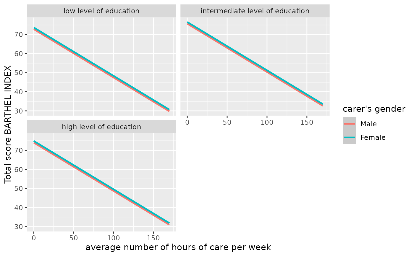
mydf <- predict_response(fit, terms = c("c12hour", "c161sex", "c172code"))

ggplot(mydf, aes(x = x, y = predicted, colour = group)) +
  stat_smooth(method = "lm") +
  facet_wrap(~facet, ncol = 2) +
  labs(
    x = get_x_title(mydf),
    y = get_y_title(mydf),
    colour = get_legend_title(mydf)
  )
#> `geom_smooth()` using formula = 'y ~ x'


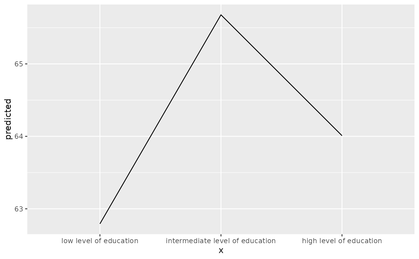
# adjusted predictions, a list of data frames (one data frame per term)
eff <- ggeffect(fit)
eff
#> $c12hour
#> # Predicted values of Total score BARTHEL INDEX
#> 
#> c12hour | Predicted |       95% CI
#> ----------------------------------
#>       0 |     75.44 | 73.25, 77.63
#>      20 |     70.38 | 68.56, 72.19
#>      45 |     64.05 | 62.39, 65.70
#>      65 |     58.98 | 57.16, 60.81
#>      85 |     53.92 | 51.71, 56.12
#>     105 |     48.85 | 46.15, 51.55
#>     125 |     43.79 | 40.52, 47.06
#>     170 |     32.39 | 27.74, 37.05
#> 
#> 
#> Not all rows are shown in the output. Use `print(..., n = Inf)` to show
#>   all rows.
#> 
#> $neg_c_7
#> # Predicted values of Total score BARTHEL INDEX
#> 
#> neg_c_7 | Predicted |       95% CI
#> ----------------------------------
#>       6 |     78.07 | 75.01, 81.14
#>       8 |     73.51 | 71.14, 75.88
#>      12 |     64.39 | 62.73, 66.04
#>      14 |     59.82 | 57.91, 61.73
#>      16 |     55.26 | 52.79, 57.73
#>      20 |     46.13 | 42.16, 50.10
#>      22 |     41.57 | 36.78, 46.36
#>      28 |     27.88 | 20.55, 35.22
#> 
#> 
#> Not all rows are shown in the output. Use `print(..., n = Inf)` to show
#>   all rows.
#> 
#> $c161sex
#> # Predicted values of Total score BARTHEL INDEX
#> 
#> c161sex | Predicted |       95% CI
#> ----------------------------------
#>       1 |     64.09 | 60.69, 67.49
#>       2 |     64.96 | 63.07, 66.86
#> 
#> 
#> $c172code
#> # Predicted values of Total score BARTHEL INDEX
#> 
#> c172code                        | Predicted |       95% CI
#> ----------------------------------------------------------
#> low level of education          |     62.79 | 59.21, 66.38
#> intermediate level of education |     65.68 | 63.55, 67.81
#> high level of education         |     64.01 | 60.14, 67.88
#> 
#> 
#> attr(,"class")
#> [1] "ggalleffects" "list"        
#> attr(,"model.name")
#> [1] "fit"
get_complete_df(eff)
#> # Predicted values of Total score BARTHEL INDEX
#> 
#> : c12hour
#> 
#> c12hour | Predicted |       95% CI
#> ----------------------------------
#>       0 |     75.44 | 73.25, 77.63
#>      35 |     66.58 | 64.91, 68.25
#>      70 |     57.71 | 55.81, 59.62
#>     100 |     50.12 | 47.55, 52.69
#>     170 |     32.39 | 27.74, 37.05
#> 
#> : c161sex
#> 
#> c12hour | Predicted |       95% CI
#> ----------------------------------
#>       1 |     64.09 | 60.69, 67.49
#>       2 |     64.96 | 63.07, 66.86
#> 
#> : c172code
#> 
#> c12hour | Predicted |       95% CI
#> ----------------------------------
#>       1 |     62.79 | 59.21, 66.38
#>       2 |     65.68 | 63.55, 67.81
#>       3 |     64.01 | 60.14, 67.88
#> 
#> : neg_c_7
#> 
#> c12hour | Predicted |       95% CI
#> ----------------------------------
#>       6 |     78.07 | 75.01, 81.14
#>      10 |     68.95 | 67.11, 70.79
#>      14 |     59.82 | 57.91, 61.73
#>      20 |     46.13 | 42.16, 50.10
#>      28 |     27.88 | 20.55, 35.22
#> 
#> 
#> Not all rows are shown in the output. Use `print(..., n = Inf)` to show
#>   all rows.

# adjusted predictions for education only, and get x-axis-labels
mydat <- eff[["c172code"]]
ggplot(mydat, aes(x = x, y = predicted, group = group)) +
  stat_summary(fun = sum, geom = "line") +
  scale_x_discrete(labels = get_x_labels(mydat))