Significance Testing Of Differences Between Predictions I: Contrasts And Pairwise Comparisons

This vignette is the first in a 3-part series:

Significance Testing of Differences Between Predictions I: Contrasts and Pairwise Comparisons
Significance Testing of Differences Between Predictions II: Comparisons of Slopes, Floodlight and Spotlight Analysis (Johnson-Neyman Intervals)
Significance Testing of Differences Between Predictions III: Contrasts and Comparisons for Generalized Linear Models

Hypothesis testing for categorical predictors

A reason to compute adjusted predictions (or estimated marginal means) is to help understanding the relationship between predictors and outcome of a regression model. In particular for more complex models, for example, complex interaction terms, it is often easier to understand the associations when looking at adjusted predictions instead of the raw table of regression coefficients.

The next step, which often follows this, is to see if there are statistically significant differences. These could be, for example, differences between groups, i.e. between the levels of categorical predictors or whether trends differ significantly from each other.

The ggeffects package provides a function, test_predictions(), which does exactly this: testing differences of adjusted predictions for statistical significance. This is usually called contrasts or (pairwise) comparisons, or marginal effects (if the difference refers to a one-unit change of predictors). This vignette shows some examples how to use the test_predictions() function and how to test wheter differences in predictions are statistically significant.

First, different examples for pairwise comparisons are shown, later we will see how to test differences-in-differences (in the emmeans package, also called interaction contrasts).

Note: An alias for test_predictions() is hypothesis_test(). You can use either of these two function names.

Summary of most important points:

Contrasts and pairwise comparisons can be used to test if differences of predictions at different values of the focal terms are statistically significant or not. This is useful if "group differences" are of interest.
test_predictions() calculates contrasts and comparisons for the results returned by predict_response() .
It is possible to calculate simple contrasts, pairwise comparisons, or interaction contrasts (difference-in-differences). Use the test argument to control which kind of contrast or comparison should be made.
If one or more focal terms are continuous predictors, contrasts and comparisons can be calculated for the slope, or the linear trend of those predictors.

Within `episode`, do levels differ?

We start with a toy example, where we have a linear model with two categorical predictors. No interaction is involved for now.

We display a simple table of regression coefficients, created with model_parameters() from the parameters package.

library(ggeffects)
library(parameters)
library(ggplot2)

set.seed(123)
n <- 200
d <- data.frame(
  outcome = rnorm(n),
  grp = as.factor(sample(c("treatment", "control"), n, TRUE)),
  episode = as.factor(sample(1:3, n, TRUE)),
  sex = as.factor(sample(c("female", "male"), n, TRUE, prob = c(0.4, 0.6)))
)
model1 <- lm(outcome ~ grp + episode, data = d)
model_parameters(model1)
#> Parameter       | Coefficient |   SE |        95% CI | t(196) |     p
#> ---------------------------------------------------------------------
#> (Intercept)     |       -0.08 | 0.13 | [-0.33, 0.18] |  -0.60 | 0.552
#> grp [treatment] |       -0.17 | 0.13 | [-0.44, 0.09] |  -1.30 | 0.197
#> episode [2]     |        0.36 | 0.16 | [ 0.03, 0.68] |   2.18 | 0.031
#> episode [3]     |        0.10 | 0.16 | [-0.22, 0.42] |   0.62 | 0.538

Predictions

Let us look at the adjusted predictions.

my_predictions <- predict_response(model1, "episode")
my_predictions
#> # Predicted values of outcome
#> 
#> episode | Predicted |      95% CI
#> ---------------------------------
#> 1       |     -0.08 | -0.33, 0.18
#> 2       |      0.28 |  0.02, 0.54
#> 3       |      0.02 | -0.24, 0.28
#> 
#> Adjusted for:
#> * grp = control

plot(my_predictions)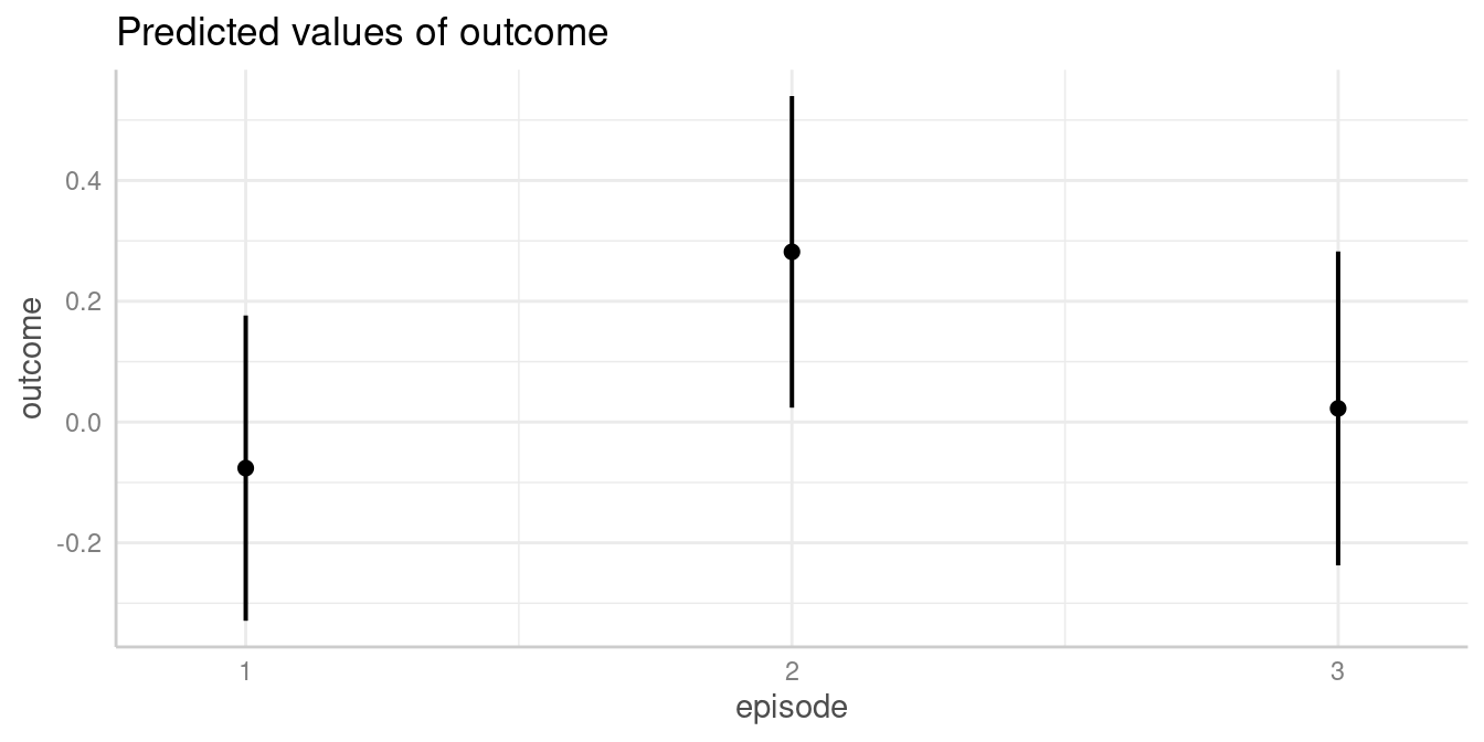

We now see that, for instance, the predicted outcome when espisode = 2 is 0.28.

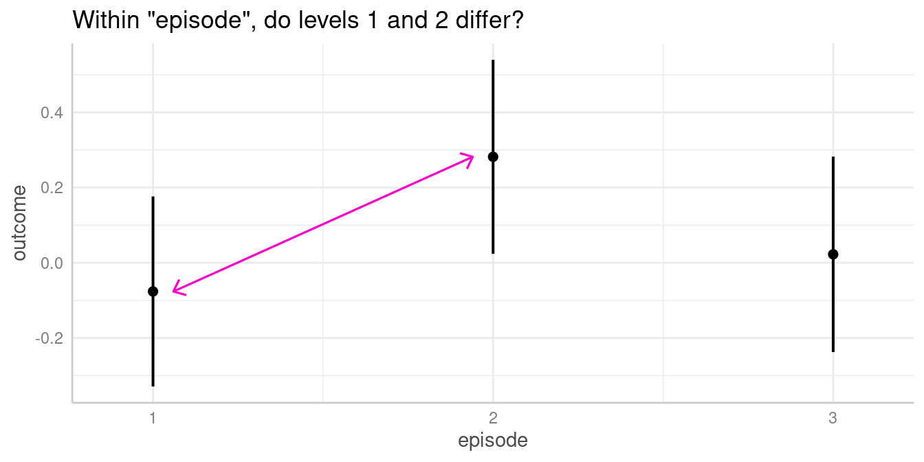
Pairwise comparisons

We could now ask whether the predicted outcome for episode = 1 is significantly different from the predicted outcome at episode = 2.

To do this, we use the test_predictions() function. This function, like predict_response(), either accepts the model object as first argument, followed by the focal predictors of interest, i.e. the variables of the model for which contrasts or pairwise comparisons should be calculated; or you can pass the results from predict_response() directly into test_predictions(). This is useful if you want to avoid specifying the same arguments again.

By default, when all focal terms are categorical, a pairwise comparison is performed. You can specify other hypothesis tests as well, using the test argument (which defaults to "pairwise", see ?test_predictions). For now, we go on with the simpler example of contrasts or pairwise comparisons.

# argument `test` defaults to "pairwise"
test_predictions(model1, "episode") # same as test_predictions(my_predictions)
#> # Pairwise comparisons
#> 
#> episode | Contrast |       95% CI |     p
#> -----------------------------------------
#> 1-2     |    -0.36 | -0.68, -0.03 | 0.031
#> 1-3     |    -0.10 | -0.42,  0.22 | 0.538
#> 2-3     |     0.26 | -0.06,  0.58 | 0.112

For our quantity of interest, the contrast between episode 1-2, we see the value -0.36, which is exactly the difference between the predicted outcome for episode = 1 (-0.08) and episode = 2 (0.28). The related p-value is 0.031, indicating that the difference between the predicted values of our outcome at these two levels of the factor episode is indeed statistically significant.

Since the terms argument in test_predictions() works in the same way as for predict_response(), you can directly pass “representative values” via that argument (for details, see this vignette). For example, we could also specify the levels of episode directly, to simplify the output:

test_predictions(model1, "episode [1:2]")
#> # Pairwise comparisons
#> 
#> episode | Contrast |       95% CI |     p
#> -----------------------------------------
#> 1-2     |    -0.36 | -0.68, -0.03 | 0.031

In this simple example, the contrasts of both episode = 2 and episode = 3 to episode = 1 equals the coefficients of the regression table above (same applies to the p-values), where the coefficients refer to the difference between the related parameter of episode and its reference level, episode = 1.

To avoid specifying all arguments used in a call to predict_response() again, we can also pass the objects returned by predict_response() directly into test_predictions().

pred <- predict_response(model1, "episode")
test_predictions(pred)
#> # Pairwise comparisons
#> 
#> episode | Contrast |       95% CI |     p
#> -----------------------------------------
#> 1-2     |    -0.36 | -0.68, -0.03 | 0.031
#> 1-3     |    -0.10 | -0.42,  0.22 | 0.538
#> 2-3     |     0.26 | -0.06,  0.58 | 0.112

Does same level of episode differ between groups?

The next example includes a pairwise comparison of an interaction between two categorical predictors.

model2 <- lm(outcome ~ grp * episode, data = d)
model_parameters(model2)
#> Parameter                     | Coefficient |   SE |        95% CI | t(194) |     p
#> -----------------------------------------------------------------------------------
#> (Intercept)                   |        0.03 | 0.15 | [-0.27, 0.33] |   0.18 | 0.853
#> grp [treatment]               |       -0.42 | 0.23 | [-0.88, 0.04] |  -1.80 | 0.074
#> episode [2]                   |        0.20 | 0.22 | [-0.23, 0.63] |   0.94 | 0.350
#> episode [3]                   |       -0.07 | 0.22 | [-0.51, 0.37] |  -0.32 | 0.750
#> grp [treatment] × episode [2] |        0.36 | 0.33 | [-0.29, 1.02] |   1.09 | 0.277
#> grp [treatment] × episode [3] |        0.37 | 0.32 | [-0.27, 1.00] |   1.14 | 0.254

Predictions

First, we look at the predicted values of outcome for all combinations of the involved interaction term.

my_predictions <- predict_response(model2, c("episode", "grp"))
my_predictions
#> # Predicted values of outcome
#> 
#> grp: control
#> 
#> episode | Predicted |       95% CI
#> ----------------------------------
#> 1       |      0.03 | -0.27,  0.33
#> 2       |      0.23 | -0.08,  0.54
#> 3       |     -0.04 | -0.36,  0.28
#> 
#> grp: treatment
#> 
#> episode | Predicted |       95% CI
#> ----------------------------------
#> 1       |     -0.39 | -0.74, -0.04
#> 2       |      0.18 | -0.18,  0.53
#> 3       |     -0.09 | -0.39,  0.21

plot(my_predictions)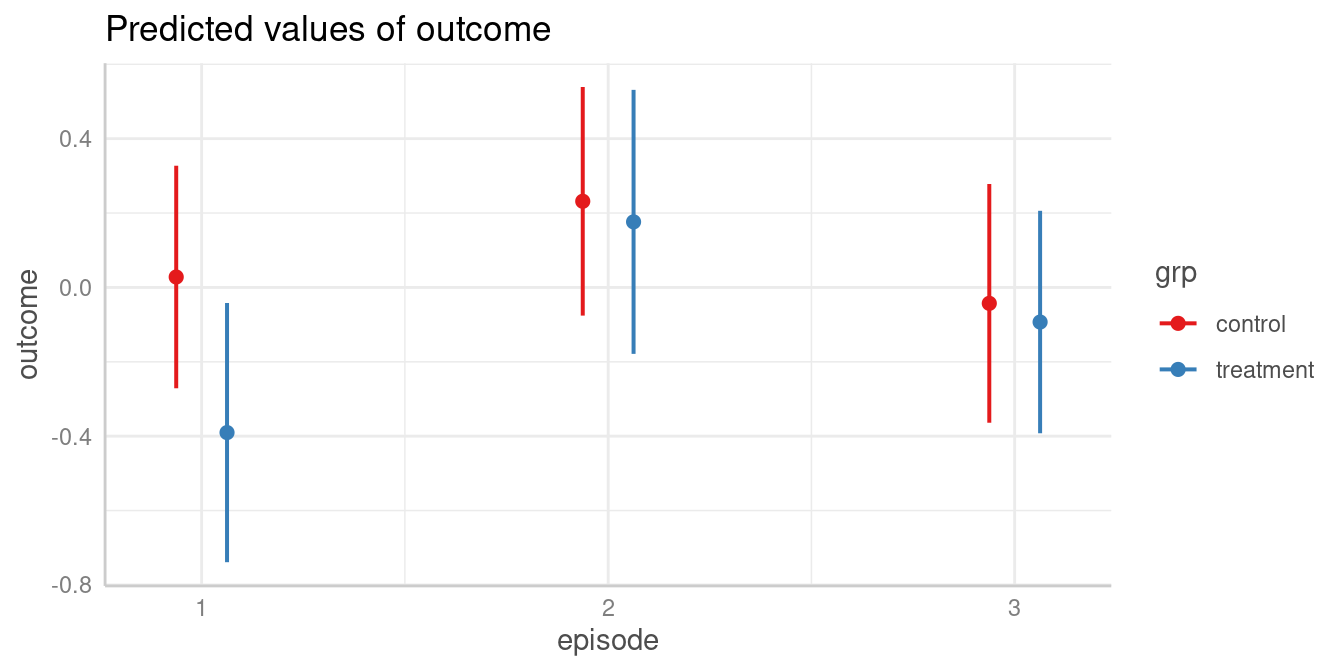

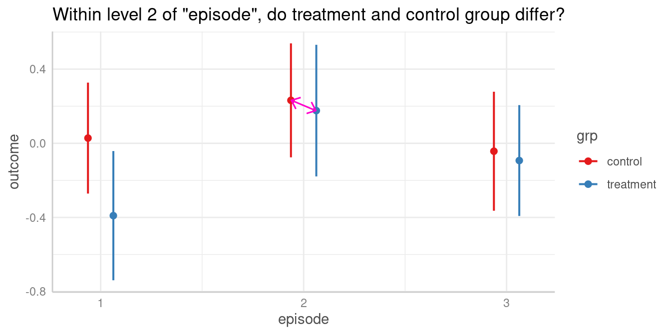
Pairwise comparisons

We could now ask whether the predicted outcome for episode = 2 is significantly different depending on the level of grp? In other words, do the groups treatment and control differ when episode = 2?

Again, to answer this question, we calculate all pairwise comparisons, i.e. the comparison (or test for differences) between all combinations of our focal predictors. The focal predictors we’re interested here are our two variables used for the interaction.

# we want "episode = 2-2" and "grp = control-treatment"
test_predictions(model2, c("episode", "grp"))
#> # Pairwise comparisons
#> 
#> episode |                 grp | Contrast |       95% CI |     p
#> ---------------------------------------------------------------
#> 1-2     |     control-control |    -0.20 | -0.63,  0.23 | 0.350
#> 1-3     |     control-control |     0.07 | -0.37,  0.51 | 0.750
#> 1-1     |   control-treatment |     0.42 | -0.04,  0.88 | 0.074
#> 1-2     |   control-treatment |    -0.15 | -0.61,  0.32 | 0.529
#> 1-3     |   control-treatment |     0.12 | -0.30,  0.54 | 0.573
#> 2-3     |     control-control |     0.27 | -0.17,  0.72 | 0.225
#> 2-1     |   control-treatment |     0.62 |  0.16,  1.09 | 0.009
#> 2-2     |   control-treatment |     0.06 | -0.41,  0.52 | 0.816
#> 2-3     |   control-treatment |     0.32 | -0.10,  0.75 | 0.137
#> 3-1     |   control-treatment |     0.35 | -0.13,  0.82 | 0.150
#> 3-2     |   control-treatment |    -0.22 | -0.70,  0.26 | 0.368
#> 3-3     |   control-treatment |     0.05 | -0.39,  0.49 | 0.821
#> 1-2     | treatment-treatment |    -0.57 | -1.06, -0.07 | 0.026
#> 1-3     | treatment-treatment |    -0.30 | -0.76,  0.16 | 0.203
#> 2-3     | treatment-treatment |     0.27 | -0.19,  0.73 | 0.254

For our quantity of interest, the contrast between groups treatment and control when episode = 2 is 0.06. We find this comparison in row 8 of the above output.

As we can see, test_predictions() returns pairwise comparisons of all possible combinations of factor levels from our focal variables. If we’re only interested in a very specific comparison, we have two options to simplify the output:

We could directly formulate this comparison as test. To achieve this, we first need to create an overview of the adjusted predictions, which we get from predict_response() or test_predictions(test = NULL).
We pass specific values or levels to the terms argument, which is the same as for predict_response().

Option 1: Directly specify the comparison

# adjusted predictions, compact table
test_predictions(model2, c("episode", "grp"), test = NULL)
#> episode |       grp | Predicted |       95% CI |     p
#> ------------------------------------------------------
#> 1       |   control |      0.03 | -0.27,  0.33 | 0.853
#> 2       |   control |      0.23 | -0.08,  0.54 | 0.139
#> 3       |   control |     -0.04 | -0.36,  0.28 | 0.793
#> 1       | treatment |     -0.39 | -0.74, -0.04 | 0.028
#> 2       | treatment |      0.18 | -0.18,  0.53 | 0.328
#> 3       | treatment |     -0.09 | -0.39,  0.21 | 0.540

In the above output, each row is considered as one coefficient of interest. Our groups we want to include in our comparison are rows two (grp = control and episode = 2) and five (grp = treatment and episode = 2), so our “quantities of interest” are b2 and b5. Our null hypothesis we want to test is whether both predictions are equal, i.e. test = "b2 = b5". We can now calculate the desired comparison directly:

# compute specific contrast directly
test_predictions(model2, c("episode", "grp"), test = "b2 = b5")
#> Hypothesis | Contrast |      95% CI |     p
#> -------------------------------------------
#> b2=b5      |     0.06 | -0.41, 0.52 | 0.816
#> 
#> Tested hypothesis: episode[2],grp[control] = episode[2],grp[treatment]

Curious how test works in detail? test_predictions() is a small, convenient wrapper around predictions() and slopes() of the great marginaleffects package. Thus, test is just passed to the hypothesis argument of those functions.

Option 2: Specify values or levels

Again, using representative values for the terms argument, we can also simplify the output using an alternative syntax:

# return pairwise comparisons for specific values, in
# this case for episode = 2 in both groups
test_predictions(model2, c("episode [2]", "grp"))
#> # Pairwise comparisons
#> 
#> episode |               grp | Contrast |      95% CI |     p
#> ------------------------------------------------------------
#> 2-2     | control-treatment |     0.06 | -0.41, 0.52 | 0.816

This is equivalent to the above example, where we directly specified the comparison we’re interested in. However, the test argument might provide more flexibility in case you want more complex comparisons. See examples below.

Do different episode levels differ between groups?

We can repeat the steps shown above to test any combination of group levels for differences.

Pairwise comparisons

For instance, we could now ask whether the predicted outcome for episode = 1 in the treatment group is significantly different from the predicted outcome for episode = 3 in the control group.

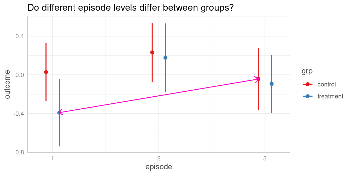
The contrast we are interested in is between episode = 1 in the treatment group and episode = 3 in the control group. These are the predicted values in rows three and four (c.f. above table of predicted values), thus we test whether "b4 = b3".

test_predictions(model2, c("episode", "grp"), test = "b4 = b3")
#> Hypothesis | Contrast |      95% CI |     p
#> -------------------------------------------
#> b4=b3      |    -0.35 | -0.82, 0.13 | 0.150
#> 
#> Tested hypothesis: episode[1],grp[treatment] = episode[3],grp[control]

Another way to produce this pairwise comparison, we can reduce the table of predicted values by providing specific values or levels in the terms argument:

predict_response(model2, c("episode [1,3]", "grp"))
#> # Predicted values of outcome
#> 
#> grp: control
#> 
#> episode | Predicted |       95% CI
#> ----------------------------------
#> 1       |      0.03 | -0.27,  0.33
#> 3       |     -0.04 | -0.36,  0.28
#> 
#> grp: treatment
#> 
#> episode | Predicted |       95% CI
#> ----------------------------------
#> 1       |     -0.39 | -0.74, -0.04
#> 3       |     -0.09 | -0.39,  0.21

episode = 1 in the treatment group and episode = 3 in the control group refer now to rows two and three, thus we also can obtain the desired comparison this way:

pred <- predict_response(model2, c("episode [1,3]", "grp"))
test_predictions(pred, test = "b3 = b2")
#> Hypothesis | Contrast |      95% CI |     p
#> -------------------------------------------
#> b3=b2      |    -0.35 | -0.82, 0.13 | 0.150
#> 
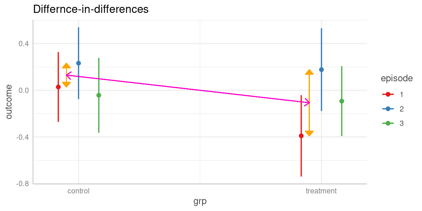
#> Tested hypothesis: episode[1],grp[treatment] = episode[3],grp[control]

Does difference between two levels of episode in the control group differ from difference of same two levels in the treatment group?

The test argument also allows us to compare difference-in-differences (aka interaction contrasts). For example, is the difference between two episode levels in one group significantly different from the difference of the same two episode levels in the other group?

As a reminder, we look at the table of predictions again:

test_predictions(model2, c("episode", "grp"), test = NULL)
#> episode |       grp | Predicted |       95% CI |     p
#> ------------------------------------------------------
#> 1       |   control |      0.03 | -0.27,  0.33 | 0.853
#> 2       |   control |      0.23 | -0.08,  0.54 | 0.139
#> 3       |   control |     -0.04 | -0.36,  0.28 | 0.793
#> 1       | treatment |     -0.39 | -0.74, -0.04 | 0.028
#> 2       | treatment |      0.18 | -0.18,  0.53 | 0.328
#> 3       | treatment |     -0.09 | -0.39,  0.21 | 0.540

The first difference of episode levels 1 and 2 in the control group refer to rows one and two in the above table (b1 and b2). The difference for the same episode levels in the treatment group refer to the difference between rows four and five (b4 and b5). Thus, we have b1 - b2 and b4 - b5, and our null hypothesis is that these two differences are equal: test = "(b1 - b2) = (b4 - b5)".

test_predictions(model2, c("episode", "grp"), test = "(b1 - b2) = (b4 - b5)")
#> Hypothesis      | Contrast |      95% CI |     p
#> ------------------------------------------------
#> (b1-b2)=(b4-b5) |     0.36 | -0.29, 1.02 | 0.277
#> 
#> Tested hypothesis: (episode[1],grp[control] - episode[2],grp[control]) = (episode[1],grp[treatment] - episode[2],grp[treatment])

Interaction contrasts can also be calculated by specifying test = "interaction". Not that in this case, the emmeans package is used an backend, i.e. test_predictions() is called with engine = "emmeans" (silently).

# test = "interaction" always returns *all* possible interaction contrasts
test_predictions(model2, c("episode", "grp"), test = "interaction")
#> # Interaction contrasts
#> 
#> episode |                   grp | Contrast |      95% CI |     p
#> ----------------------------------------------------------------
#> 1-2     | control and treatment |     0.36 | -0.29, 1.02 | 0.277
#> 1-3     | control and treatment |     0.37 | -0.27, 1.00 | 0.254
#> 2-3     | control and treatment |     0.01 | -0.64, 0.65 | 0.988

Let’s replicate this step-by-step:

Predicted value of outcome for episode = 1 in the control group is 0.03.
Predicted value of outcome for episode = 2 in the control group is 0.23.
The first difference is -0.2
Predicted value of outcome for episode = 1 in the treatment group is -0.39.
Predicted value of outcome for episode = 2 in the treatment group is 0.18.
The second difference is -0.57
Our quantity of interest is the difference between these two differences, which is 0.36. This difference is not statistically significant (p = 0.277).

Conclusion

Thanks to the great marginaleffects package, it is now possible to have a powerful function in ggeffects that allows to perform the next logical step after calculating adjusted predictions and to conduct hypothesis tests for contrasts and pairwise comparisons.

While the current implementation in test_predictions() already covers many common use cases for testing contrasts and pairwise comparison, there still might be the need for more sophisticated comparisons. In this case, I recommend using the marginaleffects package directly. Some further related recommended readings are the vignettes about Comparisons or Hypothesis Tests.

Go to next vignette: Significance Testing of Differences Between Predictions II: Comparisons of Slopes, Floodlight and Spotlight Analysis (Johnson-Neyman Intervals)

Hypothesis testing for categorical predictors

Summary of most important points:

Within episode, do levels differ?

Predictions

Pairwise comparisons

Does same level of episode differ between groups?

Predictions

Pairwise comparisons

Option 1: Directly specify the comparison

Option 2: Specify values or levels

Do different episode levels differ between groups?

Pairwise comparisons

Does difference between two levels of episode in the control group differ from difference of same two levels in the treatment group?

Conclusion

Within `episode`, do levels differ?